revised 23jul11, with Tony Winkler, 28jul11, and Zheyuan Fan, 29jul11.
 \section{Introduction}
This lesson is an expanded commentary on Hvidsten's problems 8.2.9-8.2.10
There is
a great deal of geometry hidden in these problems, which is obscured by
their brevity. The elaborations here is intended to help you use the
exercises to understand the facts and methods. A "solution" to a problem
should be more of a mini essay on what the problem means, than just cranking
out what looks like an answer to a direct question. In this spirit we proceed.
\section{Translations}
Of all the rigid motions, translation surely is the most fundamental. At
the earliest age, a child is applauded when she moves one object from
here to there. Rotations and reflections come much later. Euclid recognized
this by his second Postulate, namely that a given line segment may be
prolonged (in either direction) indefinitely. In this course, the very first
serious construction with the Geometry Explorer
(that for proving the Exterior Angle Theorem) used this principle by
transferring the notion of translation to non-Euclidean geometry.
\subsection{Vectors and Euclidean Translations}
In Calculus III you learned how vectors relate to translations in the plane.
In particular, how a vector added to every point defines the
translation. The displacement of a single point suffices to specify a
vector, and hence the entire transformation. In particular, the vector addition
properties established the translations as a group.
Here we identify and study these isometries explicitly in the non-Euclidean
context. But first we should re-examine Euclid's first Postulate.
\section{Verifying Euclid's first Postulate}
\section{Introduction}
This lesson is an expanded commentary on Hvidsten's problems 8.2.9-8.2.10
There is
a great deal of geometry hidden in these problems, which is obscured by
their brevity. The elaborations here is intended to help you use the
exercises to understand the facts and methods. A "solution" to a problem
should be more of a mini essay on what the problem means, than just cranking
out what looks like an answer to a direct question. In this spirit we proceed.
\section{Translations}
Of all the rigid motions, translation surely is the most fundamental. At
the earliest age, a child is applauded when she moves one object from
here to there. Rotations and reflections come much later. Euclid recognized
this by his second Postulate, namely that a given line segment may be
prolonged (in either direction) indefinitely. In this course, the very first
serious construction with the Geometry Explorer
(that for proving the Exterior Angle Theorem) used this principle by
transferring the notion of translation to non-Euclidean geometry.
\subsection{Vectors and Euclidean Translations}
In Calculus III you learned how vectors relate to translations in the plane.
In particular, how a vector added to every point defines the
translation. The displacement of a single point suffices to specify a
vector, and hence the entire transformation. In particular, the vector addition
properties established the translations as a group.
Here we identify and study these isometries explicitly in the non-Euclidean
context. But first we should re-examine Euclid's first Postulate.
\section{Verifying Euclid's first Postulate}
 Once we have given an interpretation of Point, Line and Incidence in a
model, we naturally want to check Euclid's first postulate, which says
that a Line connects any two Points. We have seen a geometric definition of
the Poincare model, and an analytic one. So, one can prove this postulate
is true in two ways, geometrically and analytically.
Here we do both to contrast the methods. The geometric proof uses the
Symmetry Principle and Thales' Construction but no complex numbers.
Since this approach has been omitted from this edition
of the course, you should follow
the first proof as well as you can, taking some items on faith.
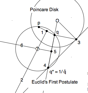
\subsection{Geometric proof}
The two Points are modelled by two points, $p,q$ in the Poincare disk.
We need a circline through $p,q$ perpendicular to the unit circle.
If the two points lie on a diameter, we're done, the diameter is the
Line they lie on. If they do not, then we need a circle through them,
which is also perpendicular to the unit circle. Here is a construction
with ruler and compass.
\begin{itemize}
\item The center of this circle must be on the perpendicular bisector of
any two points on the circle. So far we know about only two of them. So
construct the perpendicular bisector $\ell_{12}$ of the $segment(p,q)$.
\item We know such circles are symmetric with respect to the unit circle, so
we next find the symmetric point $q*=\frac{1}{\bar{q}}$ geometrically with
Thales' construction: $\ell_{q3}$ perpendicular to $\ell_{Oq}$ and
$\ell_{34}$ perpendicular to $\ell_{q3}$ meeting $\ell_{Oq}$ at $q*$.
\item The perpendicular bisector $\ell_{56}$ to $segment(q,4)$ meets the
other bisecor at the center $7$ of the required circle.
\item The portion inside the disk is the desired $L_{pq}$.
\end{itemize}
\subsection{Analytic proof}
Before we proceed with the analytic proof, we review some analytic geometry.
The equation of a circle in the complex plane can be rewritten in many
different forms. Consider the subset of circels which have the following
equivalent equations. Each version displays different
geometric properties of these circles. In particular, one of them says
that such a circle is perpendicualr to the unit circe. Therefore, the
arcs of such circles inside the unit disk are the hyperbolic lines in
the Poincare model.
\begin{eqnarray*}
z\bar{z} + \mu \bar{z} + \bar{\mu}z + 1 &=& 0 \\
|z|^2 +\mu \bar{z} + \bar{\mu}z + 1 &=& 0 \\
|z|^2 +2 \mathfrak{Re}(\mu \bar{z}) + 1 &=& 0 \\
(z + \mu)(\bar{z} +\bar{\mu}) &=& |\mu|^2 - 1 \\
|z - (-\mu))|^2 &=& ( \, \sqrt{|\mu|^2 - 1} \, \, )^2 = r^2 \\
\end{eqnarray*}
\subsubsection{Geometrical Observations}
Although the geometrical properties of such circlines are usually
presented in terms of the theory of symmetric points, it is just as
easy to derive them directly from the first equation.
Factoring the first equation (sometimes called "completing the square")
leads to the fourth
equation. The last equation,
which shows that the solution is indeed a circle with center at $-\mu$,
provided $-\mu$ lies \textit{outside} the unit circle. Otherwise the
radius, $r=\sqrt{|\mu|^2 - 1}$ would not be real. Note that the last
equation also displays the center of the circle to be at $-\mu$.
Next, consider the third equation for the point $\zeta$ where the
circle crosses the unit circle, i.e. $|\zeta|=1$ and
\begin{eqnarray*}
|\zeta|^2 +2 \mathfrak{Re}(\mu \bar{\zeta}) + 1 &=& 0 \\
2 +2 \mathfrak{Re}(\mu \bar{\zeta}) &=& 0 \\
\mathfrak{Re}(1 + \mu \bar{\zeta}) &=& 0 \\
\mathfrak{Re}(\zeta \bar{\zeta} + \mu \bar{\zeta}) &=& 0 \\
\mathfrak{Re}((\zeta + \mu) \bar{\zeta}) &=& 0 \\
\end{eqnarray*}
And the last equation says that the vector from the origin to $\zeta$ is
perpendicualr to the vector from $-\mu$ to $\zeta$ are perpendicular.
Recall that $\mathfrak{Re}( z \bar{w})$ is just a dot product of the
vectors from the origin to $z,w$ respectively. Thus the
radius of the unit circle and the radius of the circle are perpendicular
at the point where they cross. So the two circles are perpendicular,
as claimed.
\subsection{Euclid's Line Postulate}
So, given two points $p,q$ in the unit disk, to find the hyperbolic
line, $\ell_{p,q}$, we use the first form. That is, we only need to
determine the parameter $\mu$ as a function of $p,q$. But that involves
solving two equations in two unknowns as follows.
Suppose $p = x_1 + ix_1, q= y_1 + iy_2 $, and
$\mu = \mu_x + i\mu_y$ is the unknown. Then solve the two linear equation:
\begin{eqnarray*}
|z_1|^2 + \mu_x x_1 + \mu_y y_1 + 1 &=& 0 \\
|z_2|^2 + \mu_x x_2 + \mu_y y_2 + 1 &=& 0 \\
\end{eqnarray*}
for the two unknowns $\mu_x, \mu_y$. All terms are functions of the
(coordinates) of $p,q$.
Of course you remember that simulataneous linear equations have a unique
solution only if a condition is met. Check that this condition is \textbf{not}
met when $p,q$ lie on a diameter of the unit circle. Why does that issue not
matter in our argument?
Once we have given an interpretation of Point, Line and Incidence in a
model, we naturally want to check Euclid's first postulate, which says
that a Line connects any two Points. We have seen a geometric definition of
the Poincare model, and an analytic one. So, one can prove this postulate
is true in two ways, geometrically and analytically.
Here we do both to contrast the methods. The geometric proof uses the
Symmetry Principle and Thales' Construction but no complex numbers.
Since this approach has been omitted from this edition
of the course, you should follow
the first proof as well as you can, taking some items on faith.
\subsection{Geometric proof}
The two Points are modelled by two points, $p,q$ in the Poincare disk.
We need a circline through $p,q$ perpendicular to the unit circle.
If the two points lie on a diameter, we're done, the diameter is the
Line they lie on. If they do not, then we need a circle through them,
which is also perpendicular to the unit circle. Here is a construction
with ruler and compass.
\begin{itemize}
\item The center of this circle must be on the perpendicular bisector of
any two points on the circle. So far we know about only two of them. So
construct the perpendicular bisector $\ell_{12}$ of the $segment(p,q)$.
\item We know such circles are symmetric with respect to the unit circle, so
we next find the symmetric point $q*=\frac{1}{\bar{q}}$ geometrically with
Thales' construction: $\ell_{q3}$ perpendicular to $\ell_{Oq}$ and
$\ell_{34}$ perpendicular to $\ell_{q3}$ meeting $\ell_{Oq}$ at $q*$.
\item The perpendicular bisector $\ell_{56}$ to $segment(q,4)$ meets the
other bisecor at the center $7$ of the required circle.
\item The portion inside the disk is the desired $L_{pq}$.
\end{itemize}
\subsection{Analytic proof}
Before we proceed with the analytic proof, we review some analytic geometry.
The equation of a circle in the complex plane can be rewritten in many
different forms. Consider the subset of circels which have the following
equivalent equations. Each version displays different
geometric properties of these circles. In particular, one of them says
that such a circle is perpendicualr to the unit circe. Therefore, the
arcs of such circles inside the unit disk are the hyperbolic lines in
the Poincare model.
\begin{eqnarray*}
z\bar{z} + \mu \bar{z} + \bar{\mu}z + 1 &=& 0 \\
|z|^2 +\mu \bar{z} + \bar{\mu}z + 1 &=& 0 \\
|z|^2 +2 \mathfrak{Re}(\mu \bar{z}) + 1 &=& 0 \\
(z + \mu)(\bar{z} +\bar{\mu}) &=& |\mu|^2 - 1 \\
|z - (-\mu))|^2 &=& ( \, \sqrt{|\mu|^2 - 1} \, \, )^2 = r^2 \\
\end{eqnarray*}
\subsubsection{Geometrical Observations}
Although the geometrical properties of such circlines are usually
presented in terms of the theory of symmetric points, it is just as
easy to derive them directly from the first equation.
Factoring the first equation (sometimes called "completing the square")
leads to the fourth
equation. The last equation,
which shows that the solution is indeed a circle with center at $-\mu$,
provided $-\mu$ lies \textit{outside} the unit circle. Otherwise the
radius, $r=\sqrt{|\mu|^2 - 1}$ would not be real. Note that the last
equation also displays the center of the circle to be at $-\mu$.
Next, consider the third equation for the point $\zeta$ where the
circle crosses the unit circle, i.e. $|\zeta|=1$ and
\begin{eqnarray*}
|\zeta|^2 +2 \mathfrak{Re}(\mu \bar{\zeta}) + 1 &=& 0 \\
2 +2 \mathfrak{Re}(\mu \bar{\zeta}) &=& 0 \\
\mathfrak{Re}(1 + \mu \bar{\zeta}) &=& 0 \\
\mathfrak{Re}(\zeta \bar{\zeta} + \mu \bar{\zeta}) &=& 0 \\
\mathfrak{Re}((\zeta + \mu) \bar{\zeta}) &=& 0 \\
\end{eqnarray*}
And the last equation says that the vector from the origin to $\zeta$ is
perpendicualr to the vector from $-\mu$ to $\zeta$ are perpendicular.
Recall that $\mathfrak{Re}( z \bar{w})$ is just a dot product of the
vectors from the origin to $z,w$ respectively. Thus the
radius of the unit circle and the radius of the circle are perpendicular
at the point where they cross. So the two circles are perpendicular,
as claimed.
\subsection{Euclid's Line Postulate}
So, given two points $p,q$ in the unit disk, to find the hyperbolic
line, $\ell_{p,q}$, we use the first form. That is, we only need to
determine the parameter $\mu$ as a function of $p,q$. But that involves
solving two equations in two unknowns as follows.
Suppose $p = x_1 + ix_1, q= y_1 + iy_2 $, and
$\mu = \mu_x + i\mu_y$ is the unknown. Then solve the two linear equation:
\begin{eqnarray*}
|z_1|^2 + \mu_x x_1 + \mu_y y_1 + 1 &=& 0 \\
|z_2|^2 + \mu_x x_2 + \mu_y y_2 + 1 &=& 0 \\
\end{eqnarray*}
for the two unknowns $\mu_x, \mu_y$. All terms are functions of the
(coordinates) of $p,q$.
Of course you remember that simulataneous linear equations have a unique
solution only if a condition is met. Check that this condition is \textbf{not}
met when $p,q$ lie on a diameter of the unit circle. Why does that issue not
matter in our argument?
Lesson on Hyperbolic Translations
\textit{ $\C$ 2010, Prof. George K. Francis, Mathematics Department, University of Illinois} \begin{document} \maketitle
\section{Introduction}
This lesson is an expanded commentary on Hvidsten's problems 8.2.9-8.2.10
There is
a great deal of geometry hidden in these problems, which is obscured by
their brevity. The elaborations here is intended to help you use the
exercises to understand the facts and methods. A "solution" to a problem
should be more of a mini essay on what the problem means, than just cranking
out what looks like an answer to a direct question. In this spirit we proceed.
\section{Translations}
Of all the rigid motions, translation surely is the most fundamental. At
the earliest age, a child is applauded when she moves one object from
here to there. Rotations and reflections come much later. Euclid recognized
this by his second Postulate, namely that a given line segment may be
prolonged (in either direction) indefinitely. In this course, the very first
serious construction with the Geometry Explorer
(that for proving the Exterior Angle Theorem) used this principle by
transferring the notion of translation to non-Euclidean geometry.
\subsection{Vectors and Euclidean Translations}
In Calculus III you learned how vectors relate to translations in the plane.
In particular, how a vector added to every point defines the
translation. The displacement of a single point suffices to specify a
vector, and hence the entire transformation. In particular, the vector addition
properties established the translations as a group.
Here we identify and study these isometries explicitly in the non-Euclidean
context. But first we should re-examine Euclid's first Postulate.
\section{Verifying Euclid's first Postulate}
Once we have given an interpretation of Point, Line and Incidence in a
model, we naturally want to check Euclid's first postulate, which says
that a Line connects any two Points. We have seen a geometric definition of
the Poincare model, and an analytic one. So, one can prove this postulate
is true in two ways, geometrically and analytically.
Here we do both to contrast the methods. The geometric proof uses the
Symmetry Principle and Thales' Construction but no complex numbers.
Since this approach has been omitted from this edition
of the course, you should follow
the first proof as well as you can, taking some items on faith.
\subsection{Geometric proof}
The two Points are modelled by two points, $p,q$ in the Poincare disk.
We need a circline through $p,q$ perpendicular to the unit circle.
If the two points lie on a diameter, we're done, the diameter is the
Line they lie on. If they do not, then we need a circle through them,
which is also perpendicular to the unit circle. Here is a construction
with ruler and compass.
\begin{itemize}
\item The center of this circle must be on the perpendicular bisector of
any two points on the circle. So far we know about only two of them. So
construct the perpendicular bisector $\ell_{12}$ of the $segment(p,q)$.
\item We know such circles are symmetric with respect to the unit circle, so
we next find the symmetric point $q*=\frac{1}{\bar{q}}$ geometrically with
Thales' construction: $\ell_{q3}$ perpendicular to $\ell_{Oq}$ and
$\ell_{34}$ perpendicular to $\ell_{q3}$ meeting $\ell_{Oq}$ at $q*$.
\item The perpendicular bisector $\ell_{56}$ to $segment(q,4)$ meets the
other bisecor at the center $7$ of the required circle.
\item The portion inside the disk is the desired $L_{pq}$.
\end{itemize}
\subsection{Analytic proof}
Before we proceed with the analytic proof, we review some analytic geometry.
The equation of a circle in the complex plane can be rewritten in many
different forms. Consider the subset of circels which have the following
equivalent equations. Each version displays different
geometric properties of these circles. In particular, one of them says
that such a circle is perpendicualr to the unit circe. Therefore, the
arcs of such circles inside the unit disk are the hyperbolic lines in
the Poincare model.
\begin{eqnarray*}
z\bar{z} + \mu \bar{z} + \bar{\mu}z + 1 &=& 0 \\
|z|^2 +\mu \bar{z} + \bar{\mu}z + 1 &=& 0 \\
|z|^2 +2 \mathfrak{Re}(\mu \bar{z}) + 1 &=& 0 \\
(z + \mu)(\bar{z} +\bar{\mu}) &=& |\mu|^2 - 1 \\
|z - (-\mu))|^2 &=& ( \, \sqrt{|\mu|^2 - 1} \, \, )^2 = r^2 \\
\end{eqnarray*}
\subsubsection{Geometrical Observations}
Although the geometrical properties of such circlines are usually
presented in terms of the theory of symmetric points, it is just as
easy to derive them directly from the first equation.
Factoring the first equation (sometimes called "completing the square")
leads to the fourth
equation. The last equation,
which shows that the solution is indeed a circle with center at $-\mu$,
provided $-\mu$ lies \textit{outside} the unit circle. Otherwise the
radius, $r=\sqrt{|\mu|^2 - 1}$ would not be real. Note that the last
equation also displays the center of the circle to be at $-\mu$.
Next, consider the third equation for the point $\zeta$ where the
circle crosses the unit circle, i.e. $|\zeta|=1$ and
\begin{eqnarray*}
|\zeta|^2 +2 \mathfrak{Re}(\mu \bar{\zeta}) + 1 &=& 0 \\
2 +2 \mathfrak{Re}(\mu \bar{\zeta}) &=& 0 \\
\mathfrak{Re}(1 + \mu \bar{\zeta}) &=& 0 \\
\mathfrak{Re}(\zeta \bar{\zeta} + \mu \bar{\zeta}) &=& 0 \\
\mathfrak{Re}((\zeta + \mu) \bar{\zeta}) &=& 0 \\
\end{eqnarray*}
And the last equation says that the vector from the origin to $\zeta$ is
perpendicualr to the vector from $-\mu$ to $\zeta$ are perpendicular.
Recall that $\mathfrak{Re}( z \bar{w})$ is just a dot product of the
vectors from the origin to $z,w$ respectively. Thus the
radius of the unit circle and the radius of the circle are perpendicular
at the point where they cross. So the two circles are perpendicular,
as claimed.
\subsection{Euclid's Line Postulate}
So, given two points $p,q$ in the unit disk, to find the hyperbolic
line, $\ell_{p,q}$, we use the first form. That is, we only need to
determine the parameter $\mu$ as a function of $p,q$. But that involves
solving two equations in two unknowns as follows.
Suppose $p = x_1 + ix_1, q= y_1 + iy_2 $, and
$\mu = \mu_x + i\mu_y$ is the unknown. Then solve the two linear equation:
\begin{eqnarray*}
|z_1|^2 + \mu_x x_1 + \mu_y y_1 + 1 &=& 0 \\
|z_2|^2 + \mu_x x_2 + \mu_y y_2 + 1 &=& 0 \\
\end{eqnarray*}
for the two unknowns $\mu_x, \mu_y$. All terms are functions of the
(coordinates) of $p,q$.
Of course you remember that simulataneous linear equations have a unique
solution only if a condition is met. Check that this condition is \textbf{not}
met when $p,q$ lie on a diameter of the unit circle. Why does that issue not
matter in our argument?
Question 1.
Find the equation of the hyperbolic line joining
$z_1= \frac{1}{2}, z_2 = \frac{1}{2} i $.
This proves that Euclid's first postulate holds in the Poincare model of
non-Euclidean geometry.
\subsection{Comment}
Which of these two proofs do you find the easier to understand and remember?
It might depend on whether you feel more comfortable with traditional geometry,
and want to avoid using complex numbers. But in this course you need to exercise your
complex number geometry because the traditional geometric proofs become
increasingly more difficult and cumbersome. Maybe that is why, historically, it
took over two thousand years to discover non-Euclidean geometry.
\section{Verifying the remaining postulates}
We shall not verify the other postulates of Euclid. We already know they are not
adequate even for absolute geometry. In a different edition of this course,
it would be appropriate to state a complete set of axioms, similar to
Birkhoff's four axioms for Euclidean geometry. See, for example, an
excellent discussion of this issue in Appendix C of Gerard Venema,
"The Foundations of Geometry", Prentic-Hall 2005.
In the previous lesson we discussed the non-Euclidean Ruler Axiom in
the Poincare model. The negation of Playfair is built into this model from the
beginning. A nice project for you, after you have finished this course,
is to locate some other propositions from absolute geometry and verify
them in the Poincare model. For example, Circles turn out to be circles,
but their Centers are not in at their center. Note that, contrary to
Microsoft philosophy, capitalization can matter.
\section{Transitivity of the Hyperbolic Group}
One of the constant assumption Euclid makes is that there is a congruence
which takes a given point to another given point. This is called
\textit{ motion transitivity} and a translation is the easiest (though not the
only) solution of finding a hyperbolic isometry which moves one figure
to another. [Compare Hvidsten, Exercise 8.2.9]
Recall that one canonical form of elements in the hyperbolic group is given by
\[ V_{\theta, \alpha}(z)= e^{i\theta}V_\alpha(z) = e^{i\theta}\frac{z-\alpha}{\bar{\alpha}z -1}. \]
To show that one of these exists taking given a point
$p$ to another given point $q$, we might be tempted to solve
the complex equation
\[ V_{\theta,\alpha}(z_1) = z_2, \]
for the unknowns $\theta, \alpha$. Which, when the smoke clears,
becomes two equations of real numbers in 3 unknowns.
But a clever argument proves that such a solution exist without actually computing
the solution. We know that $V_\alpha(\alpha) =0 $. So the composition:
$f(z) := V_q^{-1}(V_p(p)) $ takes $ p \mapsto 0 \mapsto q $. Since a group is
closed under inverses and composition and every element has this cononical form,
we're done. Recall that these MTs are involutions, so we can drop the exponent
on the second involution. You will appreciate the elegance of this argument
if you actually do the following two, now redundant, exercises.
Question 2.
Given a MT $f(z) = \frac{az+b}{\bar{b}z+\bar{a}}$, find its canonical form.
Hint: Manipulate the fraction algebraically until it is in the proper form.
In particular, you should discover that $\alpha = -b/a$ and
$\theta = arg(-a/\bar{a})$.
Question 3.
Calculate the canonical form of the composition $V_q \circ V_p $. Hint:
Substitution yields a MT of the form $\frac{az+b}{\bar{b}z+\bar{a}}$
should determine what $a,b$ are in terms of $p,q$. Then you can apply the
result of the previous calculation.
\section{The hyperbolic translations}
There is another sort of hyperbolic isometries which have a similar form
to the involutions we have considered so far. They differ from an involution
by a rotation by $180^o$, namely
\[T_{-\alpha}(z) : = \frac{z -\alpha }{1-\bar{\alpha}z}.\]
The minus sign in front of the paramater $\alpha$ will reveal its meaning
presently.
Question 4.
Show that $T_{-\alpha}(z) = e^{i\pi}V_\alpha(z) $, while
$V_\alpha(e^{i\pi}z) = T_\alpha(z)$ .
Note that this transformation appears in Hvidsten's Exercise 8.2.10, which
has a misprint. In that exercise you will show that
\begin{eqnarray*}
T_{-\alpha}(\alpha)& =& 0 \\
T_{-\alpha}(0)& =& -\alpha \\
\mbox{For fixed point } T_{-\alpha}(z)& =& z \mbox{ if and only if} \\
z_i& =& \pm \frac{\alpha}{\bar{\alpha}} \mbox{ for } i=1,2 \\
\mbox{ unless } \alpha &=& 0 \\
\end{eqnarray*}
In particular, the two fixed points $z_1,z_2$ are \textbf{ on},
not in the unit disk. Thus these isometries have no fixed Points
in the hyperbolic plane, which is what a translation should do.
We next define
\[ T_{\alpha, \beta} := T_\beta \circ T_{-\alpha} \]
to be the hyperbolic translation that takes
$\alpha \mapsto 0 \mapsto \beta$.
To find out the form of this transformation, we continue the calculations
above to find the inverse
\[ T_{-\alpha}^{-1}(z) = T_\alpha(z) = \frac{z+\alpha}{\bar{\alpha}z + 1} .\]
Question 5.
Solve $z = \frac{w - \alpha}{1-\bar{\alpha}z}$ for
$w = \frac{z + \alpha}{\bar{\alpha}z + 1}$. How does this show that
$T_\alpha^{-1} = T_{-\alpha}.$
Finally, it would be interesting to calculate the composition
$T_{\alpha, \beta}$.
And then, to calculate the composition of two translations,
$T_{\beta, \gamma} \circ T_{\alpha, \beta}}$. But we leave this for a
later lesson in a later course.
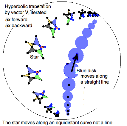
\section{Summary}
While there are important similarities between Euclidean and non-Euclidean
translations, there are even more important differences. And experiments
with the Geometry Explorer is a quick way of discovering these. The figure
for this lesson was created with GEX and iPaint to illustrate one feature.
On the one hand, the \textit{ inch worm}, namely the process of prolonging
a line segment by translation beyond itself repeatedly (and also in the
opposite direction) produces an infinite straight line in both geometries.
In the figure, the blue disk is translated along the black vector both
foreward and backward. As you can see, the extrapolated trace is a
circular arc perpendicular to the boundary of the Poincare disk. So it is
a hyperbolic line (Line!) in the model.
The colorful star is also translated by the same vector. Although it too
travels along a circular arc, this one is not perpendicular to the
boundary, and therefor not a straight Line. Since translation is an
isometry, the distance from the blue disk to the star remains constanst.
That is, the star moves along a curve which is equidistant from the the
line.
\subsection{The Saccheri Railroad}
An informative experiment for you to do with GEX is to construct a
hyperbolic railroad. The final drawing should look like
two curves equidistant from a straight line (representing the two
rails) with short, equally spaced transversals (representing the
ties). A hyperbolic railroad can run along this straight piece of
hyperbolic track. But the view from the locomotive is disconcerting.
In the classic steam locomotive, the engineer sits on left side,
looking down the left rail. He sees a curve constantly bending to the
right of the "straight ahead" direction.
You can convince yourself of this by drawing a short perpendicular
to each tie at the rail. That's "straight ahead".