2 Quadrotor Dynamics
1.1 Section Overview
Dynamics is the study of how the quadrotor actually moves about in space. Kinematics told us how to determine data once we have a location, but dynamics tells us how we get there. To model this motion, we apply the principals of Newtonian physics to determine the forces and torques that are caused by the spinning of the rotors. These are then translated into inputs; although in reality we tell the rotor to spin at a certain speed, we solve for those speeds using inputs. This makes solving the equations much simpler than it would be otherwise.
After this, we write out the equations of motion for the quadrotor. These take into account the orientation of the robot, so that regardless of what the Euler Angles are, we will be able to solve for velocities and accelerations of the model.
Finally, in preparation for writing control for the quadrotor, we must linearize the equations of motion. This is done by making approximations that allow us to simplify the equations into a form that we can use for easy application of the equations.
1.2 Forces and Torques
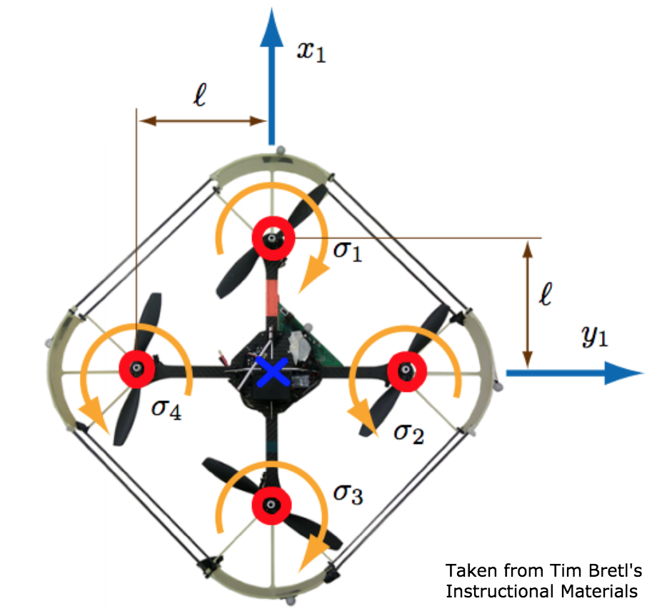
The forces produced by the spinning rotors of a quarotor are proportional to the rotor speed squared by a factor \( k_f \). Likewise, reaction torques due to the friction of air on the blades is proportional to the rotor speed squared by a factor \( k_m \). If we take body axes for a quadrotor as seen in the picture below, then a simple application of physics will determine all of the forces and torques on the body.

In particular, using right hand rule, we see that the torque about the x axis is \( \tau_x = l{k_f}((\sigma_4)^2 - (\sigma_2)^2) \), about the y axis is \( \tau_y = l{k_f}((\sigma_1)^2 - (\sigma_3)^2) \), and about the z axis is \( \tau_z = k_m((\sigma_2)^2 + (\sigma_4)^2 - (\sigma_1)^2 - (\sigma_3)^2) \). Additionally forces in the x and y directions are 0, while in the z direction it is \( f^1_{rotors} = k_f((\sigma_1)^2 + (\sigma_2)^2 + (\sigma_3)^2 + (\sigma_4)^2) \) (ignoring gravity for now).
1.3 Inputs
As mentioned in the section overview, it is easier to solve for inputs to the system, rather than individual rotor speeds. Once we have solved for those inputs in terms of the seperate rotor speeds, it is a simple matter of inversing the transformation so that we have a method to solve for rotor speeds in terms of inputs. That relationship can be seen below
$$\begin{bmatrix}u_1\\u_2\\u_3\\u_4\end{bmatrix} = W\begin{bmatrix}(\sigma_1)^2\\(\sigma_2)^2\\(\sigma_3)^2\\(\sigma_4)^2\end{bmatrix}\\
W = \begin{bmatrix}
0&-lk_f&0&lk_f\\
lk_f&0&-lk_f&0\\
-k_m&k_m&-k_m&k_m&\\
k_f&k_f&k_f&k_f
\end{bmatrix}$$
where u1 is torque about the x axis, u2 is torque about the y axis, u3 is torque about the z axis, and u4 if force in the body z direction. Notice that these are the same equations we solved for above. This can be inverted in order to solve for rotor speeds in terms of inputs, as shown below.
The importance of this is that in a real life scenario, we can solve for inputs, and then command rotor speeds based on those inputs. This sets us up to write our equations of motion in terms of inputs.
1.4 Equations of Motion
As mentioned above, the equations of motion are what show how the quadrotor will move in space. As we will see, they are determined based off of the inputs to the system, as well as the current state of the quadrotor. In their vector form, the eqations are given as
\begin{align}
\dot{\textbf{q}} &= \textbf{v}\\
\dot{\textbf{v}} &= \textbf{f}/m\\
\dot{\boldsymbol{\theta}} &= S\boldsymbol{\omega}\\
\boldsymbol{\tau} &= J\dot{\boldsymbol{\omega}} + \hat{\boldsymbol{\omega}}J{\boldsymbol{\omega}}
\end{align}
which are derived from Newton's laws of linear and rotational motion. Note the rotation of the body forces into the world frame before the addition of gravity. Also note the additional term in the torque equation, which accounts for body rotations. These can be written in the scalar equation form, as seen below.
\begin{align}
\dot{q}_1 &= v_1\\
\dot{q}_2 &= v_2\\
\dot{q}_3 &= v_3\\
\dot{v}_1 &= \frac{-u_4}{m}(c_1s_2c_3 + s_1s_3)\\
\dot{v}_2 &= \frac{-u_4}{m}(s_1s_2c_3 - c_1s_3)\\
\dot{v}_3 &= \frac{-u_4}{m}(c_2c_3) + g\\
\dot{\theta}_1 &= \frac{s_3}{c_2}w_2 + \frac{c_3}{c_2}w_3\\
\dot{\theta}_2 &= c_3w_2 - s_3w_3\\
\dot{\theta}_3 &= w_1 + \frac{s_2s_3}{c_2}w_2 + \frac{s_2c_3}{c_2}w_3\\
\dot{w}_1 &= \frac{u_1 - w_2w_3(J_3 - J_2)}{J_1}\\
\dot{w}_2 &= \frac{u_2 - w_1w_3(J_1 - J_3)}{J_2}\\
\dot{w}_3 &= \frac{u_3 - w_1w_2(J_2 - J_1)}{J_3}\\
\end{align}
where
$$f = {R^0_1}{f^1_{rotors}} + \begin{bmatrix}0\\0\\mg\end{bmatrix}$$
$${R^0_1} = \begin{bmatrix}
c_1c_2&c_1s_2s_3-s_1c_3&c_1s_2c_3 + s_1s_3\\
s_1c_2&s_1s_2s_3+c_1c_3&s_1s_2c_3 - c_1s_3\\
-s_2&c_2s_3&c_2c_3
\end{bmatrix}$$
$$f^1_{rotors} = \begin{bmatrix}0\\0\\-u_4\end{bmatrix}$$
From these, we see that we have 12 nonlinear differential equations in terms of 16 parameters. In the next section, we will see how linearizing these equations can simplify the experessions in order to represent the equations in matrix form.
1.5 Linearization
The expressions above are messy. They are nonlinear, which makes them incredibly difficult to solve. It would behoove us to linearize them - this will make the equations easier to represent and solve for using matrices.
In order to linearize an equation, we will use a first order taylor approximation. This represents the nonlinear component as a nominal value plus an additional term based on the derivative of the function, seen in the equation below.
$$h(x + {\delta}x) \approx h(x) + ({\nabla_x}h(x)){\delta}x$$
In our case, we want the quadrotor's default state to be hover. In other words, velocity, Euler angles, angular rates, and torques are all 0 while the upward force matches the force from gravity. This is called the condition that the quation is linearized about. See below for an example of linearization
\begin{align}
\dot{\theta}_2 &= c_3w_2 - s_3w_3\\
\dot{({\theta_2} + \delta\theta)} &= (\overline{c_3}\overline{w_2} - \overline{s_3}\overline{w_3}) - \overline{s_3}\overline{w_2}{\delta}\theta_3 +\overline{c_3}\overline{w_3}{\delta}\theta_2 + \overline{c_3}{\delta}w_2 + \overline{s_3}{\delta}w_3\\
\overline{\theta} &= 0, \overline{w} = 0, \overline{u_4} = mg, etc...\\
\dot{\delta\theta_2} &= (0 - 0) - 0 + 0 + {\delta}w_2 + 0\\
\dot{\delta\theta_2} &= {\delta}w_2
\end{align}
The result of applying these approximations to each function can be seen below. For the sake of brevity, the exact calculations have been left out. Suffice to say that those twelve nonlinear equations simplify down into 12 much simpler linear ones via this method.
\begin{align}
\dot{{\delta}q_1} &= {\delta}v_1\\
\dot{{\delta}q_2} &= {\delta}v_2\\
\dot{{\delta}q_3} &= {\delta}v_3\\
\dot{{\delta}v_1} &= -g{\delta}\theta_2\\
\dot{{\delta}v_2} &= g{\delta}\theta_3\\
\dot{{\delta}v_3} &= -\frac{1}{m}{\delta}u_4\\
\dot{{\delta}\theta_1} &= {\delta}w_3\\
\dot{{\delta}\theta_2} &= {\delta}w_2\\
\dot{{\delta}\theta_3} &= {\delta}w_1\\
\dot{{\delta}w_1} &= \frac{1}{J_1}{\delta}u_1\\
\dot{{\delta}w_2} &= \frac{1}{J_2}{\delta}u_2\\
\dot{{\delta}w_3} &= \frac{1}{J_3}{\delta}u_3\\
\end{align}
Implicit in this model is the assumption that the values that we linearize about is small. This can potentially be dangerous. If we make this assumption and encounter big angles, our simulated behavior and expectations of what will happen could be vastly different than what actually happens. This could result in catastrophic failure in a real scenario!
However for us this model is just fine. It will allow us to simulate the behavior of the quadrotor effectively, which is what we will explore further in the next chapter. For now, we will simply present the state-space form of these equations. Don't feel like you must understand this quite yet, but recognize that we have simply taken the twelve equations above and written them in matrix notation.
\begin{align}
\dot{\boldsymbol{\delta}\textbf{x}} = A\boldsymbol{\delta}\textbf{x} + B\boldsymbol{\delta}\textbf{u}\\
\end{align}
\begin{align}
A &= \begin{bmatrix}
0&0&0&1&0&0&0&0&0&0&0&0\\
0&0&0&0&1&0&0&0&0&0&0&0\\
0&0&0&0&0&1&0&0&0&0&0&0\\
0&0&0&0&0&0&0&{-g}&0&0&0&0\\
0&0&0&0&0&0&0&0&{g}&0&0&0\\
0&0&0&0&0&0&0&0&0&0&0&0\\
0&0&0&0&0&0&0&0&0&0&0&1\\
0&0&0&0&0&0&0&0&0&0&1&0\\
0&0&0&0&0&0&0&0&0&1&0&0\\
0&0&0&0&0&0&0&0&0&0&0&0\\
0&0&0&0&0&0&0&0&0&0&0&0\\
0&0&0&0&0&0&0&0&0&0&0&0
\end{bmatrix}\\
\\
B &= \begin{bmatrix}
0&0&0&0\\
0&0&0&0\\
0&0&0&0\\
0&0&0&0\\
0&0&0&0\\
0&0&0&{-\frac{1}{m}}\\
0&0&0&0\\
0&0&0&0\\
0&0&0&0\\
\frac{1}{J_1}&0&0&0\\
0&\frac{1}{J_2}&0&0\\
0&0&\frac{1}{J_3}&0
\end{bmatrix}\\
\\
\boldsymbol{\delta}\textbf{x} &= \begin{bmatrix}
\dot{{\delta}q_1}\\
\dot{{\delta}q_2}\\
\dot{{\delta}q_3}\\
\dot{{\delta}v_1}\\
\dot{{\delta}v_2}\\
\dot{{\delta}v_3}\\
\dot{{\delta}\theta_1}\\
\dot{{\delta}\theta_2}\\
\dot{{\delta}\theta_3}\\
\dot{{\delta}w_1}\\
\dot{{\delta}w_2}\\
\dot{{\delta}w_3}
\end{bmatrix}\\
\\
\boldsymbol{\delta}\textbf{u} &= \begin{bmatrix}{\delta}u_1\\{\delta}u_2\\{\delta}u_3\\{\delta}u_4\end{bmatrix}
\end{align}
1.6 Explore and beyond - Animation
Explore the dynamics of a quadrotor. Use this simulation to apply varius forces to each rotor, and then apply a single time step of the equations of motion and see what happens. This might show you how difficult it is to get the quadrotor to do what you would like it to!
