For the following discussion, we will suppose that we are trying to numerically solve a scalar system (to solve vector systems, apply these methods componentwise) that is described as follows:

The objective of numerical methods is to find a sequence such that

where dt is called the time step of the approximation, and n is a natural number. I will be discussing integration schemes, which are concerned with how to proceed get the next value of the approximate sequence from the previous values. This is analogous to integrating the differential equation, and is as opposed to something like a spectral or finite-difference method, where the differential equation is approximated by a set of simultaneous linear equations in points all throughout the domain. Note that integration methods require a system of first order ODEs, so if you're trying to solve a higher order system, it is necessary to introduce new variables until everything is in the first order.

Integration methods are most appropriate for my particular problem for a number of reasons. First, it is nice to watch the dynamical system evolve as it is solved, second, it does not require programming with matrix mathematics, and third, because it is simpler to implement nonlinear differential equations with integration methods (in fact, it's really no harder than with linear equations, so long as you can solve for the first derivatives).

a) Euler's method. This is the simplest method of integration, and the one most often employed by the unititiated. The sequence proceeds as follows:

This can be thought of as being analogous to the "left rectangle method", which is familiar from Riemann integration.

b) Runge-Kutta method (RK). This method is similar in principle to Euler's method, in that the (n+1)th term of the approximating sequence is only a function of the (n)th term. The difference is that where Euler's method only uses the value of g at the left point in the interval, RK explores its behaviour throughout the interval. This extra information makes it more accurate - consider, for example, trapezoidal integration. It is easy to see that by evaluating the derivative in the middle of the interval, one will generally get a better estimate than by evaluating at either end. RK takes this idea and expands on it (in fact, trapezoidal integration is a special case of second-order RK inteagration).

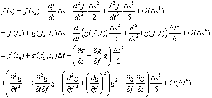
In order to understand how RK works, let us go back to the beginning. Taylor expand f about the nth time value, and substitute g for derivatives:

Now, consider Euler's method (which is supposed to approximated f):

One can see that the mapping and the function agree to the first order of dt, so that the difference is of order dt squared. Accordingly, for example, if one halfs the time step of Euler integration, one can expect the error in each step to reduce by a factor of one fourth. This difference is called the "local truncation error".

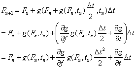
Now, consider a trapezoidal scheme:

so that

Now, in this case

The approximation now agrees up to second order. I mentioned before that trapezoidal integration is a special case of second-order RK (one can see now that "second order" refers to the power of dt that is in agreement with the actual function). In general,

agrees with the Taylor expansion up to second order if

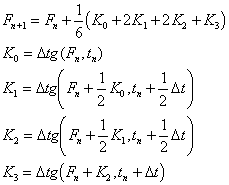
Such a technique can be generalized to give even higher orders of accuracy. The algebra is swampy, but fortunately somebody has already done it. In particular, a mapping that is fourth order accurate is given by:

It is this RK mapping that I implemented in my code. Note that every time step of RK4 requires the evaluation of g four times, which is computationally expensive. However, it has the benefit of only requiring knowledge about one value of F, as opposed to the next method.

c) Adams-Bashforth (AB)

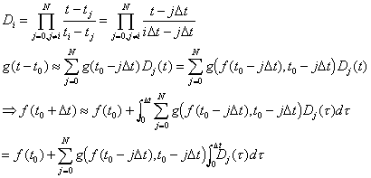
AB methods rely on the notion of polynomial fits, and one's ability to integrate polynomials exactly. Notice that although one knows g as a function of two arguments, in reality it is only a function of time, since f is a function of time. Of course, we don't know how f depends on time (that is what we are trying to find out!). However, given past data that tells how g has depended on time, one can fit the points to a polynomial which can be integrated explicitly:

This is particularly nice, since the coeffecients

can be calculated beforehand, and will show up as nothing more than constants multiplying past values of g. In particular,

agrees with f up to an error term on the order of dt to the fourth, i.e., it is fourth-order.

This is computationally faster than RK, since one can use work that is already done - the evaluation of the past derivatives. However, one has to get started somehow, since the next term in the sequence is now a function not only of its immediate predecessor, but four of its predecessors. In order to begin AB4, I used RK4 four times, and then proceeded with AB4 for the remainder.

Ryan Giordano

rgiordan@uiuc.edu