Models for non-Euclidean Gemetry
\textit{$\C$ 2010, Prof. George K. Francis, Mathematics Department,
University of Illinois}
\begin{document}
\maketitle
\section{Introduction}
As mentioned several times, Hilbert established a set of axioms for
both Euclidean and non-Euclidean geometry. These axiom sets differ only in
the Parallel Postulate as formulated by Playfair. By showing that both
Euclidean and non-Euclidean geometries
have models in Cartesian (analytic) geometry, he proved that the Parallel
Postulate is \textit{independent} from absolute geometry. This finally settled the
2200 year old controversy going back to Euclid.
In the previous section, we showed how a model for a Euclidean axiom system,
namely Birkhoff's, can be constructed in Cartesian geometry. We will accept
the much more difficult theorem stated above. It is more important for you
to understand how to use the models to discover and prove theorems in non-Euclidean geometry, than to develop non-Euclidean geometry
\textit{synthetically} as Gauss, Bolyai and Lobachevsky did.
But even that is not possible to do rigorously in an introductory course. Instead we will
pick out \textit{certain aspects} of this study, because it illustrates
the relevant methods and ideas.
In particular, many of you are taking MA402 because you will, when you are
high school teachers, have to teach an approach to non-Euclidean geometry
that happens to be favored by the author of whatever textbook
your school district favors.
In order to prepare you to do this, we will consider several approaches
that could be taken, but only their beginnings. Hvidsten's text follows \texbf{all} approaches just beyond where your high school text is likely to stop. Unless you are very short of cash, I suggest you keep Hvisdsten's book for future reference.
In this course we will use the approach of Hvidsten's Chapter 8,
but only the first four sections (17 pages !). This choice is
dictated by the following considerations:
\begin{itemize}
\item It uses the algebra of \textit{complex numbers}
to treat the geometry of the Euclidean plane in which the
models for non-Euclidean geometry are placed.
\item Most future high school teachers graduate from college
without having taken a course on complex numbers.
By at least learning the geometry of complex numbers, which is much easier
than the differential and integral calculus of complex numbers,
this loss is mitigated.
\item Hvidsten treats both Euclidean and
non-Euclidean plane geometry from
the \textit{transformational} viewpoint. This is the way
all modern higher geometry has been treated for the past century,
high school textbooks notwithstanding.
\item While this is the \textit{steepest} approach to the
plateau we need to achieve, it is also the \textit{shortest} path there.
This makes the best use of the pedagogical resources of a
university math course.
\end{itemize}
\subsection{The Role of GEX}
Although the Geometry Explorer software is a superb tool for experimentation,
it cannot provide proofs for any theorems. The operation of GEX is based
on the analytic geometry that does provide rigorous proofs.
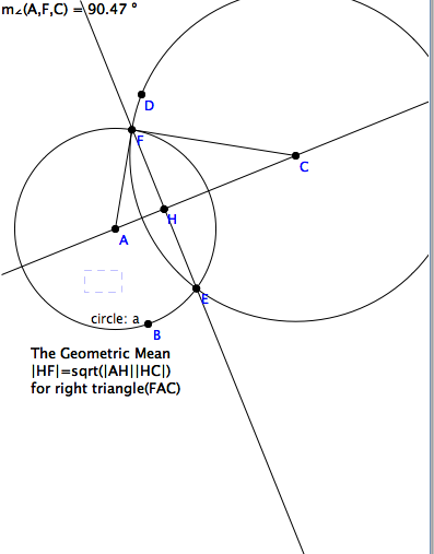
For example (see the figure above), start with two circles with centers
and a radial points, hencforth denoted by $crcl(A,|AF|), crcl(C,|CD|)$
respectively. Locate their intersections and drop the perpendicular
from one to the line connecting the centers of the circle. Note that the
perpendicular passes through the other intersection.
Complete $\triangle FAC $ and measure $\angle F$. Wiggle one circle until
this angle is as close to a right angle as possible. Now focus your
attention on this \textit{Thales Figure}.
The three right triangles in Thales' Figure are similar. The proof of
this fundamental theorem is developed in an Exercise below. Conclude that
\begin{eqnarray*}
\mbox{short/long =} |AH|/|FH| & = & |FH|/|HC| \\
|AH||HC| & = & |FH|^2 \\
\mbox{short/hypot =} |AH|/|AF| & = & |AF|/|AC| \\
|AH||AC| & = & |AF|^2 \mbox{= radius circle}_a^2 \\
|AH| &= & \frac{r_a^2}{|AC|} \\
c &= & \frac{r_a^2}{h} \\
\end{eqnarray*}
The two points $H$ and $C$ are said to be \textit{inverses} relative to
to $crcl{A;B}$. Notice that if $crcl{A,B}$ is the unit circle, then
the distances from the origin, $ hc = 1$ are inverses in the sense of
\textit{reciprocals.}
\subsection{Construction of the Inverse of an Inside Point}
Given $crcl(A,D)$ and any point $H$ inside the circle. To construct
its inverser, $C$, reconstruct Thales' Figure from different starting
points. Erec the perpendicular to $ray(A;H)$ at $H$, intersecting
the circle at $F$. Now construct a right angle to $AF$ at $F$. The
inverse point $F$ is where the other leg of the \textit{gnomon} crosses
the $ray(A;H)$.
\subsection{Construct the Inverse of an Outside Point.}
To do this construction precisely, with ruler and compass or with GEX,
is not entirely trivial. But for an adequate approximate solution with
a \textit{gnomon} is very easy. Given $crcl(O,R)$ (change of notation
is intentional.) Let $Y$ be a point outside the circle. Position your
gnomon with one edge going through $O$, the other edge going through
$Y$, and the right angled corner on the circle. This is the Thales
right triangle, with hypotenuse on the line $\ell_{OY}$. Drop the
altitude (again by placing your gnomon intelligently) to $X$ on
the hypotenuse. That is the inverse point.
To do this precisely we apply the classical construction the Greeks
called \textit{constructing the mean and extreme ratio.}
\subsection{Construction of the Mean and Extreme}
Given two lengths (represented by segments) $x,y$, find their geometric mean $ h = \sqrt{xy} $.
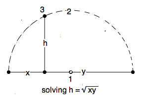
We saw one solution to this above. But here is a clean, simple one, using
just Thales' Figure. Bisect a segment of lenght $ x+y $, erect a semicircle
abover this segment as diameter, and erect the perpendicular to it at the
point separating the diameter into lengths $x$ and $y$. Where the altitude
crosses the semicircle is the right angle of the inscribed right angle.
Hence it is the geometry mean.
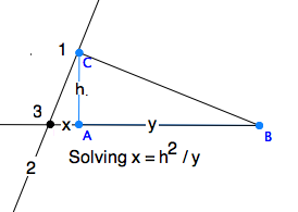
Given two lengths (represented by segments) $h,y$, find the length $x$,
solving the equation $ h = \sqrt{xy}$.
(1) On a segment of length
$y$, erect a seqment of length $h$ perpendicular to it. In the figure this
point is $C$. (2) Erect the perpendicular to $BC$ at $C$ to (3) where it
crosses the linge $\ell_{AB}$. This completes Thales Figure once again,
and we have found $x$.
These two constructions are useful to find inverses of points in a given
circle, whether the starting point is inside or outside. Be sure you
complete this construction in your journal.
\section{The Poincare Disk Model}
The document, titled
"The
Poincar\'e Models of the Hyperbolic Plane" ,
provided here in .pdf format, uses the concept of \textit{inversion in
circles}, which is a generalization of \textit{reflection in lines}.
Hvidsten introduces this idea in Chapter 2 and it is the basis of his exposition of non-Euclidean geometry in Chapter 7.
In Chapter 8, Hvidsten
covers much of the same material using a different appraoch, one using
complex numbers. Although we shall take the \textit{Complex Number approach},
it is useful for you to have some familiarity with the
\texit{Cartesian approach} using inversions in circles.
The reason for taking the complex number approach is that it is no more
difficult to learn a bit of the geometry of complex numbers than to work
one's way through inversive geometry in a purely analytic way. It is one
of the more spectacular successes in mathematics, that complex numbers,
originally invented to solve polynomial equations (like the familiar
quadratic formula) should be so well suited to describe plane
geometry as well.
\subsection{What you should study now.}
Chapter 8 is quite difficult and requires time. So we shall not
pursue the .pdf notes on the Poincare models beyond sections 1
and 2, but only up to section 2.1, for the time being.
\section{The Klein Disk Model}
The document, titled
"The Beltrami-Klein
Model of Hyperbolic Geometry" ,
provided here in .pdf format, takes a different approach than the
previous, one proper to \texit{synthetic geometry}. Analytic (or
Cartesian) geometry was such a huge success in mathematics after the
17th century, that the beauty of the classical way of doing geometry
in the style of Euclid was neglected. Geometers coined the term
\textit{synthetic} as opposed to \textit{analytic} geometry for the
classical approach. And synthetic geometry involves construction with
ruler and compass. So here we present non-Euclidean geometry in the
style that was more familiar to the actual discoverers of non-Euclidean
geometry, Gauss, Lobachevsky and Bolyai.
\subsection{Euclid's First Postulate}
The very first construction in Euclid is to connect two Points with a Line.
(Note the capitals refer to the primitives in an axiomatic system, to be
interpereted in the model.)
In the Klein model, this is trivial, because, by definition the
Line connecting two Points is just the secant of the disk through the
two points, excluding the end points. In the Poincar\'e disk, the
Line $\ell_AB$ is the arc of a circle through the points which is
also perpendicular to the circle. The critical theorem to use here is
the following, which we shall prove later.
\begin{theorem}
Given a circle $K$, another circle $C$ is perpendicular to $K$
if and only if it is its own inverse in $K$.
\end{theorem}
So now, given Points $P,Q$ in the Poincare model, we invert one of them,
to get $P'$ outside the Poincare circle. Recall the high school geometry
construction of a circle through three given points $P,Q,P'$. Its center
is where the perpendicular bisector of secant $PQ$ meets the perpendicular
bisector of $P'Q$.
\subsection{Euclid's Third Postulate}
Solving the problem of dropping a Perpendicular from a Point to a Line
depends first and foremost on the interpretation of Perpendicular in
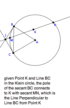
the model. For the Klein model, this is fairly odd. In the picture, let
$crcl(A,|AB|)$ be the Klein disk. The secant $BC$ is a Line. Construct
tangents to the circle at the endpoints of the secant, intersecting at
$J$ in the figure. This is called the \texit{pole of the secant}.
We define another secant, say $MN$ to be a Line Perpendicular to the
original Line, as long as its extensions outside goes through the pole $J$.
\textbf{Exercise}
Show by experimentation that if Line $MN$ is Perpendicular to $BC$, as
just defined, then Line $BC$ is also Perpendicular to Line $MN$. This
reflexivity of ``being perpendicular" is not at all obvious.
\subsection{What you should study now.}
From the .pdf notes titled the
\textit{Beltrami-Klein Projective Model}, you need only study
the first two sections for now.