Circle in Turtle Geometry
9sep15
\begin{document}
\maketitle
\section{Introduction}
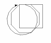
This elementary lesson on Python with turtle geometry motivates the definition
of a circle as a plane curve with constant curvature. It includes a detailed
reading of a Python journal which created this figure.
\section{Python Journaling}
Here is a (somewhat edited) transcript,
circle-journal an immediate mode
Python session. Such a \texti{Python Journal} is a recording of what
was typed and entered into a Python session. You can just follow the
steps in the circle-journal yourself. And you can read the following
lesson if you aren't sure you understand what you're doing.
\subsection{Check your Python}
First, check that your computer has a working Python installation.
Open a command shell and enter the phrase following the dollar sign
in the example below. Python will answer with something like what
is written below the input line, ending with the prompt >>>. You
then enter the phrase following the prompt.
\$ python
Python 2.4.3 (#1, Jan 10 2007, 12:05:23)
[GCC 4.0.1 (Apple Computer, Inc. build 5250)] on darwin
Type "help", "copyright", "credits" or "license" for more information.
> > > import turtle
There is no response by Python to this lasst command. You have told Python
to use the turtle libraries (in Pythonspeak, this is called the
"turtle module"). If do get a reply from Python here, then Python cannot
find this module. And you cannot continue this lesson, until you install
this module. This means, your current Python needs to be augmented with
software you can obtain elsewhere. But that is another story not told here..
To see the entire "vocabulary" of the turtle-module,
enter the following command. Note that the name \texttt{dir}, which stands
for "directory", is the name of a function, and therefore it must be
followed by the parentheses proper to functional notation in mathematics.
The vocabulary only tells you the names. It does not tell you how to use
these. For example, \texttt{cos} obviously stands for the cosine function, and
so you would type \texttt{cos(42)}. But you still not know whether this cosine
fuction is in degrees or radians. You can find out, but how will be
told later. For the time being, use functions you are told about here.
>>> dir(turtle)
['Error', 'Pen', 'RawPen', 'Tkinter', '__builtins__', '__doc__',
'__file__', '__name__', '_canvas', '_getpen', '_pen', '_root',
'acos', 'asin', 'atan', 'atan2', 'backward', 'ceil', 'circle',
'clear', 'color', 'cos', 'cosh', 'degrees', 'demo', 'down', 'e',
'exp', 'fabs', 'fill', 'floor', 'fmod', 'forward', 'frexp', 'goto',
'heading', 'hypot', 'ldexp', 'left', 'log', 'log10', 'modf', 'pi',
'position', 'pow', 'radians', 'reset', 'right', 'setheading',
'setx', 'sety', 'sin', 'sinh', 'sqrt', 'tan', 'tanh', 'tracer',
'up', 'width', 'window_height', 'window_width', 'write']
It is neither necessary nor advisable to understand all of these. You can,
of course, experiment with any of the words which don't begin with a
double underscore. The ones we're interested for this lesson are
are \texttt{forward, right, reset}.
\texttt{ >>> turtle.forward(50) }
The turtle module now opens a screen on your computer. That is, it invokes
another module called "Tkinter" which "knows" how to draw in the plane.
Moreover, we want to abbreviate the command to something simpler. We can
write an alias for the words, but not for the parentheses. The latter indicate
the the words refer to a function, and the input to the function, in this
case, was 50.
>>> \texttt{ fd = turtle.forward} \n
>>> \texttt{ fd(50) }\n
>>> \texttt{ turtle.right(90)} \n
>>> \texttt{ fd(50)} \n
>>>\texttt{ rt=turtle.right \n
>>> \texttt{ rt(90)} \n
>>> \texttt{ fd(50)} \n
>>> \texttt{ rt(90)} \n
>>> \texttt{ fd(50})
Well, wasn't that fun? But tedious. Let's check the directory for
a nother useful function, one that puts everything back to the beginning.
\texttt{>>> dir(turtle)}
Same output as before.
\texttt{>>> turtle.reset()}
Aha, that's what we want. Let's call it "zap" for short.
>>> \texttt{zap=turtle.reset}
We next "define" our own function to draw a square. We'll call it
\texttt{ square} and we insert a placeholder for the side-length of the square.
The word \texttt{ dis} can be anything you like, but best not to confuse Python
by using one of the words already in its vocabulary.
When you end the line with a colon, Python presents you with another
prompt, the tripple of dots. There you MUST indent a number of spaces.
Although you may, you should NEVER use (TAB).
Here I used my usual two spaces. One space is too short to see, more
spaces is a waste of effort.
To tell Python you're done writing, enter a blank line. Python will
return to the standard >>> prompt.
\texttt{ >>> def square(dis): }\n
\texttt{ ... \ \ fd(dis) }\n
\texttt{ ... \ \ rt(ang) }\n
\texttt{ ... \ \ fd(dis) }\n
\texttt{ ... \ \ rt(ang) }\n
\texttt{ ... \ \ fd(dis) }\n
\texttt{ ... \ \ rt(ang) }\n
\texttt{ ... \ \ fd(dis) }\n
\texttt{ ... \ \ rt(ang) }\n
\texttt{ ... }\n
\texttt{ >>> square(96) }
Always check that something you've just defined does what you expect it
to do.
We now speed up. Here is a loop. Note that loop counter, a dummy variable
here called "i" because it's easy to type, takes on five values: 0,1,2,3,4.
We do not use it for anything. We just want five loops. Clearly 4 would
have sufficed.
\texttt{ >>> for i in range(5): }\n
\texttt{ ... \ \ fd(dist) }\n
\texttt{ ... \ \ rt(ang) }\n
\texttt{ ... }
Now we are ready to do some serious programming.
\texttt{ >>> zap() }
A polygon has three attributes, number of sides, lenght of side, and
angle.
\texttt{ >>> def poly(nn, dis, ang): }\n
\texttt{ ... \ \ for i in range(nn): }\n
\texttt{ ... \ \ \ \ fd(dis) }\n
\texttt{ ... \ \ \ \ rt(ang) }\n
\texttt{ ... }\n
Can you write out in words what this program does? It's easier to see
it do it, isn't it?
\texttt{ >>> poly(4,96,90) }\n
\texttt{ >>> poly(8,43,45) }\n
You are welcome to double the number of sides, and halve the side
lenght and turning angle. But you'll get a cramp typing. Let's do this:
\texttt{ >>> num=4 }\n
\texttt{ >>> dist=96 }\n
\texttt{ >>> angl=90 }\n
\texttt{ >>> zap() }\n
\texttt{ >>> poly(num,dist,angl) }\n
\texttt{ >>> poly(2*num,dist/2,angl/2) }\n
\texttt{ >>> poly(5*num,dist/5,angl/5) }\n
What's going on here? Write a short essay into your journal on this
experiment.
\section{Mathematics}
Ever since Euclid in the year -300 school children were taught that
a circle is the locus of points equidistant from its center point.
But every child knows that a circle is a curve which is round, like
a wheel. How to reconcile this? The above experiment suggest a way.
Note that in each iteration, although we halve the distance moved, $ds$,
we also halve the angle turned, $d\phi$. Thus the ratio,
$\frac{d\phi}{ds} =$ is kept constant. In the limit, as $ds \rightarrow 0$,
this ratio is called the \textit{ curvature} of the curve along which the
turtle moved. Incidentally, the reciprocal of the curvature, called the
\textit{ radius of curvature} is the, as you might expect, the radius
of the circle.
\textbf{Exercise:} If you have taken calculus and learned a different formula
for the curvature of a, say the graph of a function $y=f(x)$, the you should
(try) to see that the two expressions are equivalent by differentiating
the formulas that change rectangular to polar coordinates. The best answer
is written up by Eric Weissstein in his Mathworld webpages: \url{http://mathworld.wolfram.com/Curvature.html}
\end{document}