A Short Lesson on Quadric Surfaces
17nov10 revised 17aug11, 25aug11 with the class.\begin{document} \maketitle In 3D, this \[ ax^2 +by^2 + cz^2 + dxy + eyz +fzx +gx +hy + kz + m=0 \] is the formula for a \textit{quadric surface}. The quadric surface is the locus of points $(x,y,z)$ that satisfy the equation. The 10 parameters $a,b,c,....,m$ determine the shape of the quadric. We would like to know how they do this.
 \section{The 1D quadratic equation}
In high school, you studied the familiar \textit{ quadratic equation} $ ax^2 +bx +c =0$
to death. It has only 1 variable, $x$, but 3 parameters, $a,b,c$.
But we're not quite done with it. It has to serve us as the humble bottom rung in the
\textit{ dimensional ladder}, sometimes called a dimensional \textit{dialectic}
in honor of Plato's method of reaching a glimpse of the Ideas. It is a process of
seeing into higher dimensions by carefully developing analogies from lower dimensions.
In this case, we wish to have a peek into the 10D parameter space to find which
structures correspond to which quadrics.
Unfortunately, in 1D the entire solution is described by the familiar
quadratic equation:
\[ ax^2 +bx +c =0 \iff x = \frac{-b \pm \sqrt{b^2 - 4ac}}{2a} \]
which consists of a single point when $b^2 = 4ac$, and has two or no (real) solutions,
depending on whether $b^2 \gt \mbox{ or } \lt 4ac$.
The surface, $b^2=4ac$, is called the \textit{discriminant} of the quadratic equation, and for
$(a,b,c)$ on the discriminant surface, there is only one solution.
On one side of the surface there are two solutions. On the other side
of the surface there are no solution.
\subsection{What the discriminant looks like}
To graph the discriminant surface in 3-dimensional $abc$-space using DPGraph,
we have to rename the coordinates to $x,y,z$ because DPGraph expects you to do
that. Then, DPGraph shows $y^2=4xz$ very well.
\section{The 1D quadratic equation}
In high school, you studied the familiar \textit{ quadratic equation} $ ax^2 +bx +c =0$
to death. It has only 1 variable, $x$, but 3 parameters, $a,b,c$.
But we're not quite done with it. It has to serve us as the humble bottom rung in the
\textit{ dimensional ladder}, sometimes called a dimensional \textit{dialectic}
in honor of Plato's method of reaching a glimpse of the Ideas. It is a process of
seeing into higher dimensions by carefully developing analogies from lower dimensions.
In this case, we wish to have a peek into the 10D parameter space to find which
structures correspond to which quadrics.
Unfortunately, in 1D the entire solution is described by the familiar
quadratic equation:
\[ ax^2 +bx +c =0 \iff x = \frac{-b \pm \sqrt{b^2 - 4ac}}{2a} \]
which consists of a single point when $b^2 = 4ac$, and has two or no (real) solutions,
depending on whether $b^2 \gt \mbox{ or } \lt 4ac$.
The surface, $b^2=4ac$, is called the \textit{discriminant} of the quadratic equation, and for
$(a,b,c)$ on the discriminant surface, there is only one solution.
On one side of the surface there are two solutions. On the other side
of the surface there are no solution.
\subsection{What the discriminant looks like}
To graph the discriminant surface in 3-dimensional $abc$-space using DPGraph,
we have to rename the coordinates to $x,y,z$ because DPGraph expects you to do
that. Then, DPGraph shows $y^2=4xz$ very well.
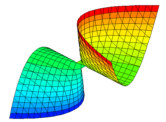
Question 1.
In DPGraph, what does the locus of the equation $y^2=4xz$ look like to you?
But because the axis of this double cone is not aligned with the
$xyz$-axes, it is easily mistaken for some other quadric.
If, however, we make the \textit{ substitution} (the $\leftarrow$ means to
replace its LHS with its RHS):
\begin{eqnarray*}
x & \leftarrow & \frac{z-x}{2}\\
y & \leftarrow & y \\
z & \leftarrow & \frac{z+x }{2} \\
\end{eqnarray*}
then we get the more recognizable equation
\[y^2=z^2-x^2 \mbox{ equivalently } x^2 +y^2 = z^2 \]
whose locus (a.k.a. solution set). We can see from the
last equation that the surface has circles of radius $|z|$ as
cross-sections parallel to the $xy$-plane.
For $x=0$ we factor \[ 0= y^2-z^2=(y-z)(y+z) \] for the equation of two crossing
lines. Thus the discriminant surface is a double cone.
Question 2.
Why does the locus of points $(z,y)$ satisfying $(z-y)(z+y) = 0$ lie on two
crossing lines? What are their equations?
\subsection{Comments for experts}
An author never quite knows whether a text will befuddle or bore the reader. Commercially
successful text books are designed to err on the side of caution. They rarely befuddle,
and so they are usually boring. So, if the above discussion is boring, here is something
for you to think about.
If we rotate these two crossing lines about the $z-axis$ then the surface so formed is a
double cone. That's obvious. But in what sense is this the "same" surface we were looking
for? The substitution above describes, in effect, a rotation of this double cone about
the y-axis (and a rescaling by factor of $\sqrt{2}$.) This is the transformation you
were taught in high school to "solve" the 2D quadratic equation we consider next.
Historically, functions, and transformations were called substitutions.
\subsection{The 2D quadratic equation}
Now, lets (try) to do the same thing in 2D. Note that the quadratic equation
from high school is just a (somewhat
very!) special case of the equation for a quadric surface (given at the
top), namely with $b=c=d=e=f=h=k=0$. If we set only those coefficients to
zero which are followed by a $z$ term, we get the
\textit{2D quadratic equation}
\[ax^2 + bxy + cy^2 + dx + ey + f =0 \].
The loci of the 2D quadratic equation
are called the \textit{ conics} because these curves are all obtained
by cutting a (double) cone in 3D by a plane (you learned
that in high school, right?).
Question 3.
Which conic is described by $1=a=e, 0=b=c=d=f$?
\subsubsection{ A more challenging question.}
Find a good web reference where you can look up which conditions on
the parameters specify what kind of conic: parabola, hyperboal, ellipse,
parallel lines, crossing lines, point, empty set. Share it with the class.
\subsection{Homogenizing equations}
One approach to solving the quadratic equation is very geometrical.
And it also happens to be a key algebraic ingredient in computer
graphics. It consists of turning the quadratic
equation into a \textit{ homogeneous} equation. We do
this by first setting a new variable $w=1$ and then mutliplying through by
1 the "right number of a number of times".
Let's see how this works in 1D.
We write $ax^2 + bxw + cw^2 = 0$. Note that there are always the same number
of variables in each term. In the first, there are two $x$'s. In the second
there is an $x$ and a $w$, and so forth.
Morevover, this is a special
case for the 2D quadratic equation ($d=e=f=0$), provided we release $w=1$ and let it be
2nd variable in 2D $xw$-space.
(Our letters may vary from paragraph to paragraph, but not their roles.
Letters at the end of the alphabet are spatial coordinates, and the parameters use
letters from the beginning of the alphabet.)
\subsection{Homogenizing the 1D quadratic equation}
We now solve the 1D homogenous quadratic equation as follows.
\[ ax^2 + bxw + cw^2 = 0.\]
If $a=0$ and $b\ne0$ (if it were, we'd have nothing to look at, right?) then the LHS factors
into $w(bx+cw)=0$, which is true if $w=0$ or if $(bx+cw)=0$, both of which are equations
of straight lines in $xw$-space. To get back to 1D, we set $w=1$ (which is still another line)
and look at the intersection the locus (loci) makes with the special line $w=1$.
If $a\ne0$ then we can "remove" it as a coefficient for the $x^2$ term simply by dividing
the equation by $a$. The RHS remains zero. And we could now rewrite the equation as
$x^2 + 2Bxw + Cw^2 =0$, explaining what the parameters $B,C$ are in terms of the original
parameters, $a,b,c$. This procedure is sometimes called "eliminating" the parameter $a$.
We don't do this here for some deeper reasons, which we'll get back to eventually.
\begin{eqnarray*}
x^2 +2\frac{b}{2a}x w+\frac{c}{a}w^2 & = & 0 \\
x^2 +2\frac{b}{2a}x w + \frac{b^2}{4a^2}w^2 & = & \left( \frac{b^2}{4a^2} - \frac{c}{a}\right)w^2 \\
\left(x + \frac{b}{2a}w \right)^2 &= & \left( \frac{\sqrt{b^2 - 4ac}}{2a}w\right)^ 2 \\
\left(x + \frac{b}{2a}w \right)^2 - \left( \frac{\sqrt{b^2 - 4ac}}{2a}w\right)^ 2 &=&0 \\
\end{eqnarray*}
\begin{eqnarray*}
\left(x + \left( \frac{b}{2a} + \frac{\sqrt{b^2 - 4ac}}{2a}\right)w \right) \left(x + \left(\frac{b}{2a} - \frac{\sqrt{b^2 - 4ac}}{2a}\right)w \right) &=& 0 \\
\end{eqnarray*}
The last line is the equation of two lines crossing at the origin in the
$x,w$-space. When we set $w=1$ again, then
these two lines cross horizontal line, $w=1$, at the two solutions
you got by solving the high school quadratic equation.
Question 4.
What was the procedure called in high school, that takes us from the first equation
to the second? Do you remember?
The foregoing was an example of how to solve an inhomogenous equation in some
number of dimensions, by solving a homogeneous equation in one dimension higher. Working in
homogenous coordinates is an essentail aspect of computer graphics as it has been in
algebraic geometry for hundreds of years.
\section{The space of lines in the plane}
Note that by solving the 1D quadratic equation in the foregoing way, we also solved the
special case of the 2D quadratic equations $ x^2 + bxy + cy^2 = 0$, only with different
letters. We next consider the ``latter half" of the entire quadratic equation, namely
the case of \textit{ linear equations} in the plane, $dx +ey +f =0$, except that we rewrite
this equation again, as $ax+by+c=0$. And, as before we homogenize the equation to,
what is in effect, the equation of a straight line through the origin in $xyw$-space.
\[ ax + by + cw = 0 \].
This time we want to know how to characterize each
line such an equation defines. In high school you knew lines by their ``point-slopes",
as in $y=mx+b$, or by two points on the line, or some other geometrical property of the line.
Now we want to understand the lines in the plane as the \textit{ points} in some space, which
we shall call the \textit{ moduli space} of lines in the plane. A more familiar names for
this, especially in physics,
might be \textit{ configuration space}.
In general the moduli space is not the same as the
\textit{ parameter space}, which here is the 3D $abc$-space.
Why is that? Because the point $(a,b,c)$
is not unique to the line. The equation $(ta)x + (tb)y +(tc) =0$ describes the exact same line,
provided that $t \ne 0$, of course. (Think: what is the locus when $t=0$.) The Greeks
would have said that it isn't the triple $(a,b,c)$ that determines the line, but its
ratio $a:b:c$. Because when we multiply by $t$ we do not change the three ratios, just
as we do not change the truth or falsehood of the equation when we test it at
a particular point $(x,y)$ in the plane.
So, what we really want to know how to imagine the space of all proportions $a:b:c$,
except $a=b=c=0$. First, we make the meaning of $a:b:c$ precise. For a century
now, mathematicians use set theory and logic for precision. That's why you had to study
Venn diagrams in high school. We define
\[ a:b:c = \{ (ta,tb,tc) | t\ne 0\} \]
and the space of all proportions as
\[ \mathcal{M} = \{ a:b:c | 0 \ne a^2+b^2+c^2\} \]
So defined, $a:b:c$ is the set of all points on a line through the origin in
3-space, except the origin itself.
Question 5.
Which lines in space have are described by these proportions $1:0:0$, $1:1:1$ and $2:0:0$?
To solve this visualization problem we shall need some topology. Since
$a:b:c = ta:tb:tc$ for all $t\ne 0$, we can \textit{ normalize} the proportion
by dividing through by $\pm r = \sqrt{a^2+b^2+c^2}$, so that
$(a/r,b/r,c/r)$ and $(-a/r,-b/r,-c/r)$ are the points on the unit sphere where
the line named by the proportion pierces the sphere. Not that these two points
are \textit{ antipodes}, just like the north and the sourth poles constitute a
pair of antipodes. Since the two antipodal points on the sphere specify the
same line, we still don't have the moduli space. We need to consider each
pair of antipodes as a single "point" in some other space.
In some circles of topology people would content themselves by saying that
the moduli space we are seeking to visualize is the unit sphere, $S^2$, with
antipodes indentified to single points, \[P^2 = S^2/(a,b,c)\sim (-a,-b,-c)\].
The letter P is for "projective plane", a concept invented by Renaissance artists
when they discovered the laws of perspective.
Because the projective plane is difficult to visualize, we proceed instead by
throwing away one of the each pair of antipodes so as to leave only one of the
two hemispheres separated by the equator, say the southern one. So now, each
point strictly below the equator corresponds to a unique line in the $xy$-plane.
For instance, the "east pole" $(0,-1,0)$ corresponds to the line with
equation $y=0$.
Question 6.
Why does the point $(-\frac{1}{\sqrt{3}},-\frac{1}{\sqrt{3}},-\frac{1}{\sqrt{3}})$
correspond to the line $x+y+1=0$ in the plane?
But on the equator we still have antipodes. For instance $(0,\pm 1,0)$
both correspond to the line $y=0$ in the plane.
We could throw away half the equator, and we would have a picture of the
moduli space. But this space has a very ``raw edge" where half the
equator used to be. So we proceed to try and suture this raw edge.
While there is a nice visualization of this
procedure, it's not the easiest to appreciate without computer graphics.
(The illiSnail animation illustrates this.)
\subsection{Werner Boy's model of Ferdinand Moebius' Surface}
Start with the sphere and decompose it into three pieces, a belt along the
equator that extends the same distance above as below the equator. What
remains are two disjoint polar caps. Every point in one cap has its antipode
in the other. So we discard one of the caps and keep the other. Just remember
we have to sew it back to the equatorial belt eventually.
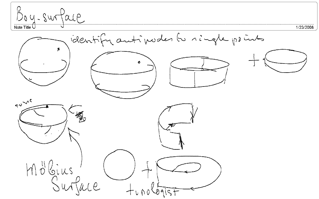 The belt also contains antipodes. This time we cut it in half, leaving an
``east strip" and and ``west strip". Again each point in one strip has
its antipode in the other (and vice versa), so we discard one of them.
We're not done. The vertical (short) cuts on the west strip are antipodes. But
now we can identify these, provided we put a half-twist into the strip. We
get a \textit{ Moebius strip}. This has a single circle for an edge, to which we
propose to glue the remaining cap. Of course we can't do that in 3-space.
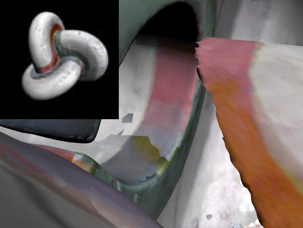
If we contort the Moebius strip and the cap just right, and allow the surface
to pass through itself, then we can, and so obtain what
is known as a \textit{ Boy surface}, because Werner Boy first figured out how
to do that.
Now we are done. We have proved that the moduli space for the lines in the
plane is a Boy surface. For entirely different reasons, it is also called
the \textit{ projective plane}. Visualizing a Boy surface is visualization problem
left for another time.
The belt also contains antipodes. This time we cut it in half, leaving an
``east strip" and and ``west strip". Again each point in one strip has
its antipode in the other (and vice versa), so we discard one of them.
We're not done. The vertical (short) cuts on the west strip are antipodes. But
now we can identify these, provided we put a half-twist into the strip. We
get a \textit{ Moebius strip}. This has a single circle for an edge, to which we
propose to glue the remaining cap. Of course we can't do that in 3-space.
If we contort the Moebius strip and the cap just right, and allow the surface
to pass through itself, then we can, and so obtain what
is known as a \textit{ Boy surface}, because Werner Boy first figured out how
to do that.
Now we are done. We have proved that the moduli space for the lines in the
plane is a Boy surface. For entirely different reasons, it is also called
the \textit{ projective plane}. Visualizing a Boy surface is visualization problem
left for another time.
 \section{Three Things Left Undone}
While we can understand the space of all lines in the plane in terms of the
projective plane (a.k.a. Moebius' Surface) we have a long way to go to imagining
the moduli space for all conics in the the plane.
And, of course, there remains the problem of quadric surfaces, which will require
another dimensional step higher. We shall leave both of these problems for
another time, and even a another course. But DPGraph is available for
experimentally exploring the world of quadrics.
\subsection{The Line at Infinity}
There is, however, one little oversight which opensw yet another door. Earlier, we
declared the points in the southern hemisphere as representing lines in the plane.
We even looked at two examples. But there is one example we overlooked. The
south pole, $(0,0,-1)$ would correspond to the homogeneous equation $ -cw = 0$
which is equivalent to $w=0$. To find the corresponding line in the $xy$-plane,
we de-homogenize by setting $w=1$, and obtain the absurdity $1=0$. This
is clearly not the equation of line in the $xy$-plane. It is, in fact, an
equation which is never true. The resolution to this paradox can proceed in
two ways. One, we throw the south pole out of the moduli space. Two, add a line
to the plane which we cannot, ordinarily, see, the \textit{ line at infinity}
in the \textit{ perspective plane.} That too, is left for a nother time,
another lesson, or even, another course.
\end{document}
\section{Three Things Left Undone}
While we can understand the space of all lines in the plane in terms of the
projective plane (a.k.a. Moebius' Surface) we have a long way to go to imagining
the moduli space for all conics in the the plane.
And, of course, there remains the problem of quadric surfaces, which will require
another dimensional step higher. We shall leave both of these problems for
another time, and even a another course. But DPGraph is available for
experimentally exploring the world of quadrics.
\subsection{The Line at Infinity}
There is, however, one little oversight which opensw yet another door. Earlier, we
declared the points in the southern hemisphere as representing lines in the plane.
We even looked at two examples. But there is one example we overlooked. The
south pole, $(0,0,-1)$ would correspond to the homogeneous equation $ -cw = 0$
which is equivalent to $w=0$. To find the corresponding line in the $xy$-plane,
we de-homogenize by setting $w=1$, and obtain the absurdity $1=0$. This
is clearly not the equation of line in the $xy$-plane. It is, in fact, an
equation which is never true. The resolution to this paradox can proceed in
two ways. One, we throw the south pole out of the moduli space. Two, add a line
to the plane which we cannot, ordinarily, see, the \textit{ line at infinity}
in the \textit{ perspective plane.} That too, is left for a nother time,
another lesson, or even, another course.
\end{document}