% Week 3 Progress Report
% Abdulmajed Dakkak
% June 27th, 2008
Saturday/Sunday
===============
Read a few papers about the LBM, HPP, and FHP CA.
Lattice Boltzmann Methods
-------------------------
A list differences between Lattice Boltzmann Methods (LBM) and regular
numerical methods are found in Chen and Dollen's paper. The differences
include:
1. The convection operator of the LBM in phase space is linear. If advection
is the same as convection, then in CFD (primarily Stam's Stable Fluids
method), one needs to use either a semi-Lagrangian scheme (which is unstable),
or, as Stam suggests, a more numerically stable technique such as the _method
of characteristics_. Advection is the term $-(\vec{u} \bullet \nabla) u$ in
the Navier-Stokes equations.
2. The incompressible Navier-Stokes equations can be derived from the nearly
incompressible limit of the LBM.
3. The LBM method utilizes a minimal set of velocities in phase space.
HPP
---
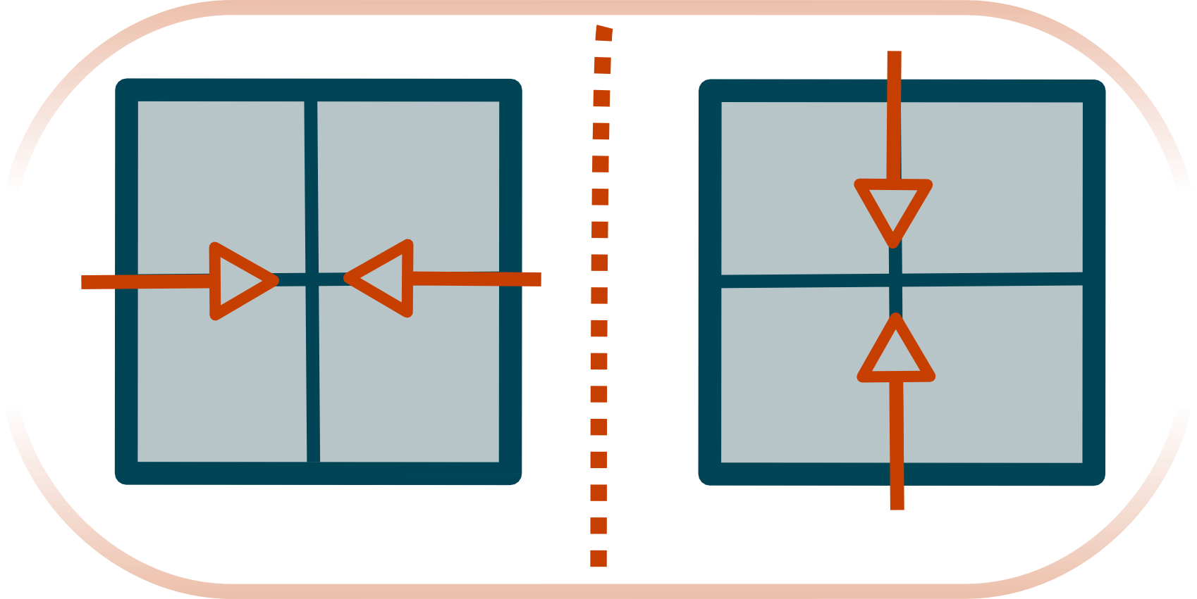
One of the first attempts to use CA to approximate NSE is called the _HPP
model_ after "Hardy-Pomeau-Pazzis", the authors of a 1973 paper describing the
model. The idea of the model is quite simple:
* Discretize the domain to a square lattice
* Only one particle found in the same vertex on the grid,
* Move particles in the same previous direction
* If a collision occurs, then the particles move in a direction perpendicular
to their entry point.
The image bellow summarizes the gist of the model
 \includegraphics[scale=0.1]{graphics/hpp.png}
While such a model is simple and ideal for 1973 (when parallel computing was
the fad), if we consider its limit, it does not approximate the NSE. This is
partly because the inadequate rotational symmetry of the square lattice
(having only $\pi/2$ symmetry).
The HPP model is still used to simulate sand mixed with water and other rigid
liquids (**need to find paper that mentioned this**).
FHP
---
In 1986 it was realized that the only two dimensional lattice that remotely
approximates the NSE was the hexagonal lattice. This model was realized by
_Frish-Hasslacher-Pomeau_ and a few months later independently by Wolfram (who
references the 1986 article in CA fluids 1). The model was extended to 3 space
by FHP in 1987.
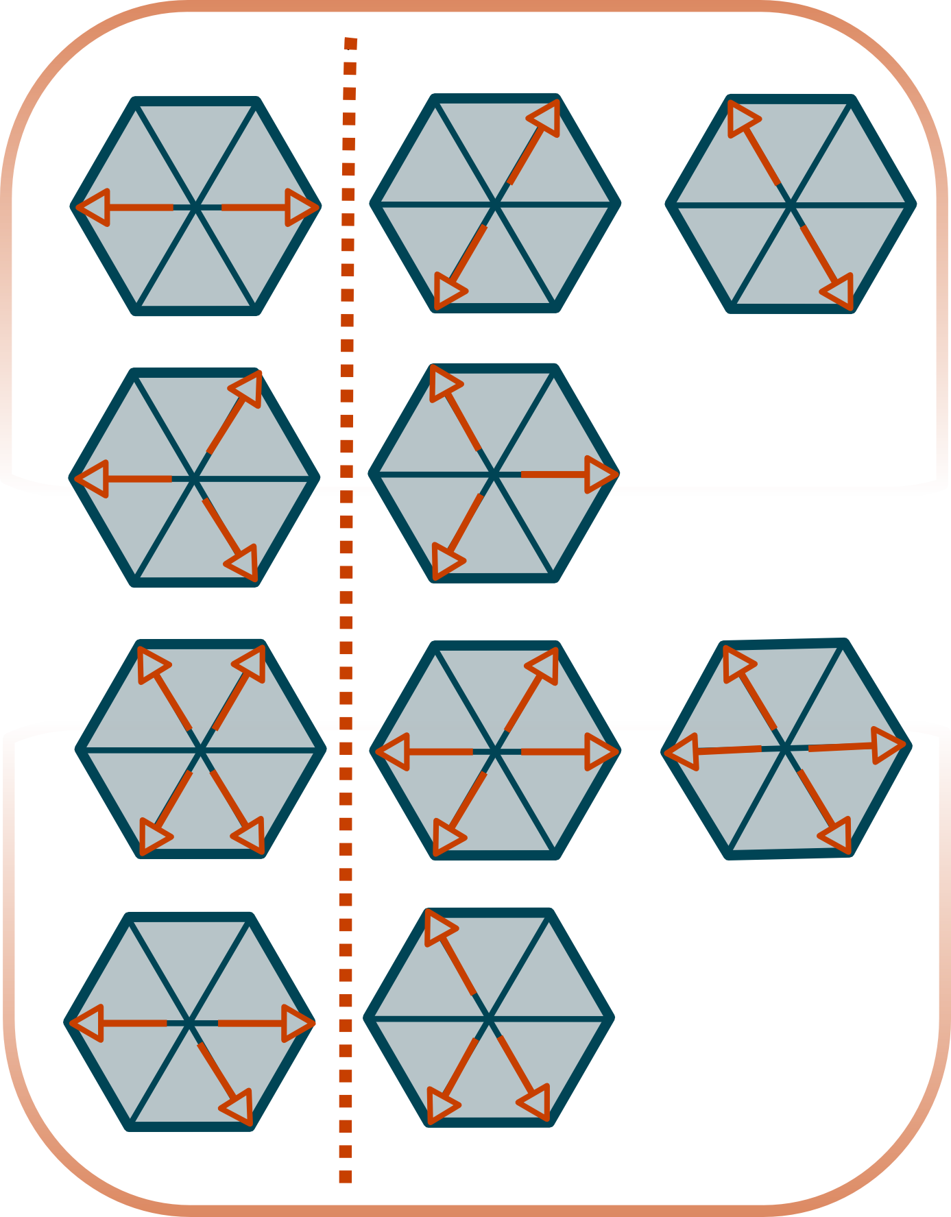
The FHP model is similar to the HPP model. Again, only one particle can be at
any position on the grid. The update rules are a bit more complex, and
described by the following figure (appears in "Lattice-gas cellular automata
and lattice Boltzmann by Dieter (springer) and page 378 in NKS).
\includegraphics[scale=0.1]{graphics/hpp.png}
While such a model is simple and ideal for 1973 (when parallel computing was
the fad), if we consider its limit, it does not approximate the NSE. This is
partly because the inadequate rotational symmetry of the square lattice
(having only $\pi/2$ symmetry).
The HPP model is still used to simulate sand mixed with water and other rigid
liquids (**need to find paper that mentioned this**).
FHP
---
In 1986 it was realized that the only two dimensional lattice that remotely
approximates the NSE was the hexagonal lattice. This model was realized by
_Frish-Hasslacher-Pomeau_ and a few months later independently by Wolfram (who
references the 1986 article in CA fluids 1). The model was extended to 3 space
by FHP in 1987.
The FHP model is similar to the HPP model. Again, only one particle can be at
any position on the grid. The update rules are a bit more complex, and
described by the following figure (appears in "Lattice-gas cellular automata
and lattice Boltzmann by Dieter (springer) and page 378 in NKS).
 \includegraphics[scale=0.1]{graphics/fhp.png}
An output is selected randomly if multiple outputs can be realized.
Papers Read
-----------
* Somers, 1993. J.A. Somers, Direct simulation of fluid flow with cellular
automata and the lattice-Boltzmann equation. Appl. Sci. Res. 51 (1993), pp.
127–133.
* CHEN, S., and G.D. DOOLEN, 1998. Lattice Boltzmann method for fluid flows.
Annu. Rev. Fluid Mech, 30, 329–364.
* Something on Rule 184 and its relation to traffic flow.
Lectures Watched
----------------
* Wolfram's NKS [lecture][mit_lecture] at MIT in 2003.
* Irving, G., Guendelman, E., Losasso, F., and Fedkiw, R. 2006. Efficient
simulation of large bodies of water by coupling two and three dimensional
techniques. In ACM SIGGRAPH 2006 Papers (Boston, Massachusetts, July 30 -
August 03, 2006). SIGGRAPH '06. ACM, New York, NY, 805-811. DOI=
http://doi.acm.org/10.1145/1179352.1141959
* Treuille, A., Lewis, A., and Popović, Z. 2006. Model reduction for
real-time fluids. In ACM SIGGRAPH 2006 Papers (Boston, Massachusetts, July
30 - August 03, 2006). SIGGRAPH '06. ACM, New York, NY, 826-834. DOI=
http://doi.acm.org/10.1145/1179352.1141962
[mit_lecture]: http://mitworld.mit.edu/video/149/
Monday
======
My first attempt to implement the FHP CA did not go anywhere because I had no
idea how to generate the hexagonal lattice. Most of the time was thus devoted
figuring out the optimal way to generate and represent the lattice.
Representing the Hexagonal Lattice
----------------------------------
While the CA is simple, I wanted to look at how to optimize my grid code as
early as possible, since it would be a bottle neck if the lattice is scarce.
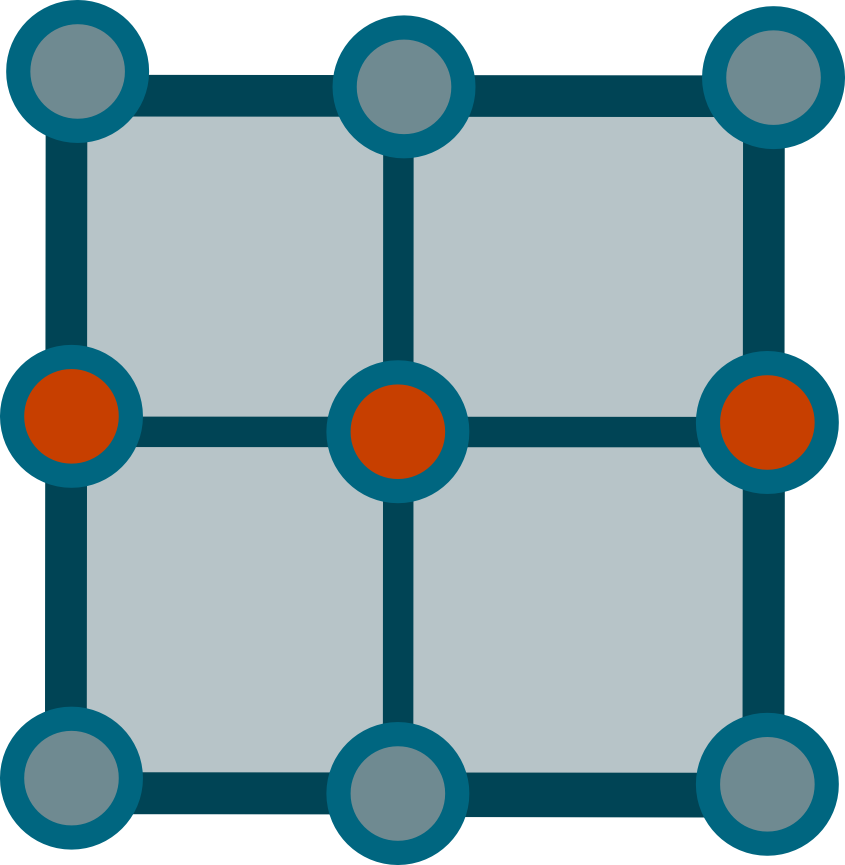
The first question was how to represent that lattice as an array. A Naive was
is to think of the two dimensional array in terms of $3 \times 3$ blocks. Each
of these blocks represents a single lattice; shown bellow.
\includegraphics[scale=0.1]{graphics/fhp.png}
An output is selected randomly if multiple outputs can be realized.
Papers Read
-----------
* Somers, 1993. J.A. Somers, Direct simulation of fluid flow with cellular
automata and the lattice-Boltzmann equation. Appl. Sci. Res. 51 (1993), pp.
127–133.
* CHEN, S., and G.D. DOOLEN, 1998. Lattice Boltzmann method for fluid flows.
Annu. Rev. Fluid Mech, 30, 329–364.
* Something on Rule 184 and its relation to traffic flow.
Lectures Watched
----------------
* Wolfram's NKS [lecture][mit_lecture] at MIT in 2003.
* Irving, G., Guendelman, E., Losasso, F., and Fedkiw, R. 2006. Efficient
simulation of large bodies of water by coupling two and three dimensional
techniques. In ACM SIGGRAPH 2006 Papers (Boston, Massachusetts, July 30 -
August 03, 2006). SIGGRAPH '06. ACM, New York, NY, 805-811. DOI=
http://doi.acm.org/10.1145/1179352.1141959
* Treuille, A., Lewis, A., and Popović, Z. 2006. Model reduction for
real-time fluids. In ACM SIGGRAPH 2006 Papers (Boston, Massachusetts, July
30 - August 03, 2006). SIGGRAPH '06. ACM, New York, NY, 826-834. DOI=
http://doi.acm.org/10.1145/1179352.1141962
[mit_lecture]: http://mitworld.mit.edu/video/149/
Monday
======
My first attempt to implement the FHP CA did not go anywhere because I had no
idea how to generate the hexagonal lattice. Most of the time was thus devoted
figuring out the optimal way to generate and represent the lattice.
Representing the Hexagonal Lattice
----------------------------------
While the CA is simple, I wanted to look at how to optimize my grid code as
early as possible, since it would be a bottle neck if the lattice is scarce.
The first question was how to represent that lattice as an array. A Naive was
is to think of the two dimensional array in terms of $3 \times 3$ blocks. Each
of these blocks represents a single lattice; shown bellow.
 \includegraphics[scale=0.05]{graphics/repr.png}
It should be easy, however, to see that such representation would waste 3
positions that the model does not care about. An alternative approach is to
remove the middle row from the representation, and concentrate on the first
and last row. We thus get the following representation
6 1
5 2
4 3
based on the following numbering scheme
\includegraphics[scale=0.05]{graphics/repr.png}
It should be easy, however, to see that such representation would waste 3
positions that the model does not care about. An alternative approach is to
remove the middle row from the representation, and concentrate on the first
and last row. We thus get the following representation
6 1
5 2
4 3
based on the following numbering scheme
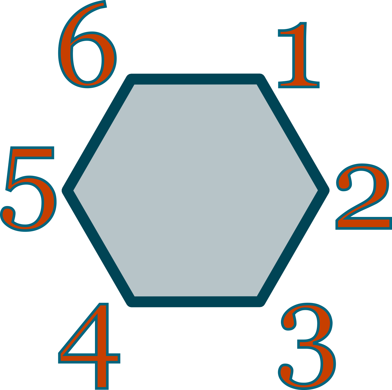 \includegraphics[scale=0.07]{graphics/g5.png}
A $3 \times 2$ block. If we then rewrite our representation in of the FHP
model using this representation we get
\includegraphics[scale=0.07]{graphics/g5.png}
A $3 \times 2$ block. If we then rewrite our representation in of the FHP
model using this representation we get
 \includegraphics[scale=0.2]{graphics/fhp2.png}
It should be noted that if we want $n^2$ lattices ($n$ rows with $n$ columns)
then we do not need a $n*3 \times n*2$ array. This can is evident if we stack
more lattices in this representation.
6 1
51 26
462 351
531 462
426 5131
35 42
4 3
Which represents the orange region found in the following pictorial
representation
\includegraphics[scale=0.2]{graphics/fhp2.png}
It should be noted that if we want $n^2$ lattices ($n$ rows with $n$ columns)
then we do not need a $n*3 \times n*2$ array. This can is evident if we stack
more lattices in this representation.
6 1
51 26
462 351
531 462
426 5131
35 42
4 3
Which represents the orange region found in the following pictorial
representation
 \includegraphics[scale=0.1]{graphics/hex.png}
This $7 \times 2$ represents on three lattice rows with one lattice per row.
We can generalize the size of the matrix to be
2*num_of_lattice_rows + 1 x num_of_lattice_columns + 1
> Note: Originally I was representing this as a $2 \times 3$ matrix
>
> 6 1 2
> 5 4 3
>
> because of some complications writing this section, however, I chose to
> switch to a $3 \times 2$ coding scheme.
Papers Read
-----------
* Ilachinski, A., (2001). Cellular Automata. City: World Scientific Publishing
Company. (Chapter on Fluids)
Tuesday
=======
Revised the representation of the lattice. Started coding the FHP model.
Code
----
* [fhp.c][tuesday-fhp](does not work)
[tuesday-fhp]: code/tuesday-fhp.c
Wednesday
=========
After talking to Dr. Francis who explained some the history behind I was
doing, I decided to go back and implement the simpler HPP model in Python, in
the end, however, it did not work.
One question that I and Dr. Francis had was what exactly did Wolfram try on
the Connection Machine. After a few hours of research, I found some
interesting information. The following is a snippet of an email exchange
between me and Dr. Francis on the topic.
This <
http://www.stephenwolfram.com/publications/articles/ca/88-cellular/1/text.html>
is about the only time wolfram mentions his work on the connection machine
in the 1980s. As to what type of method he used, one has to look elsewhere
from < http://www.longnow.org/views/essays/articles/ArtFeynman.php >
" Cellular automata started getting attention at Thinking Machines when
Stephen Wolfram, who was also spending time at the company, suggested that
we should use such automata not as a model of physics, but as a practical
method of simulating physical systems. Specifically, we could use one
processor to simulate each cell and rules that were chosen to model
something useful, like fluid dynamics. For two-dimensional problems there
was a neat solution to the anisotropy problem since [Frisch, Hasslacher,
Pomeau] had shown that a hexagonal lattice with a simple set of rules
produced isotropic behavior at the macro scale. Wolfram used this method on
the Connection Machine to produce a beautiful movie of a turbulent fluid
flow in two dimensions. Watching the movie got all of us, especially
Feynman, excited about physical simulation. We all started planning
additions to the hardware, such as support of floating point arithmetic that
would make it possible for us to perform and display a variety of
simulations in real time."
The above quote comes partly from a book called "Feynman and Computation,"
and that is the only reference to CA and fluids (or wolfram) in that book. A
more (auto)bibliographical account can be found in NKS <
http://www.wolframscience.com/nksonline/page-880b-text >
"I had always thought that cellular automata could be a way to get at
foundational questions in thermodynamics and hydrodynamics. And in mid-1985,
partly in an attempt to find uses for the Connection Machine, I devised a
practical scheme for doing fluid mechanics with cellular automata (see page
378 ). Then over the
course of that winter and the following spring I analyzed the scheme and
worked out its correspondence to the traditional continuum approach.
By 1986, however, I felt that I had answered at least the first round of
obvious questions about cellular automata, and it increasingly seemed that
it would not be easier to go further with the computational tools available.
In June 1986 I organized one last conference on cellular automata--then in
August 1986 essentially left the field to begin the development of *
Mathematica*."
He thus used the FHP model that I am trying to get to work right now. Also,
the 4D fluid simulation is called FHCP <
http://arxiv.org/abs/chao-dyn/9508001v1 >
It should also be mentioned that Wolfram patented not only the hexagonal
method for solving fluid dynamics, but the entire lattice gas method as a
whole. See patent number 4809202 <
http://www.google.com/patents?id=FF4WAAAAEBAJ&dq=U.S.+Patent+Number+4,809,202>
Code
----
* [hpp.py][hpp.py](does not work)
[hpp.py]: code/hpp.py
Thursday
========
I realized that my interpretation of the model was incorrect the entire time.
After I gave a presentation, received some helpful tips, and learned more, I
decided to start from scratch. After a few hours, I was able to correctly
implement the HPP model. The implementation, along with the algorithm, is
detailed in [HPP document][hpp.doc] posted on the website.
Code
----
* [hpp.c][hpp.c]
[hpp.c]: code/hpp.c
[hpp.doc]: ../lattice-gas/lattice-gas.html
Friday
======
Looked at how Jared Schaber, and wrote [notes][dbz]. Talked to Jonathan Manton
who described how to implement the FHP model (I wish I had that talk before,
since I figured out much of what he said the day before). Jonathan also
explained the concepts behind CUDA, compiler optimization, and a slew of other
things. He also gave me tips on how to optimize my program, while stressing
that clarity is the most important objective at the beginning.
[dbz]: ../dbz/dbz.html
Questions
=========
In _Cellular Automata Super Computers for Fluid Dynamics Modeling_ (by
Margolus) the author writes the following about implementing CA in
conventional architecture (not CAM):
> two dimensional planes are processed serially (with a substantial amount
> of pipelining); a third dimension is achieved by staking planes and
> operating on them in parallel.
The question is: how can this be achieved without running into race
conditions.
\includegraphics[scale=0.1]{graphics/hex.png}
This $7 \times 2$ represents on three lattice rows with one lattice per row.
We can generalize the size of the matrix to be
2*num_of_lattice_rows + 1 x num_of_lattice_columns + 1
> Note: Originally I was representing this as a $2 \times 3$ matrix
>
> 6 1 2
> 5 4 3
>
> because of some complications writing this section, however, I chose to
> switch to a $3 \times 2$ coding scheme.
Papers Read
-----------
* Ilachinski, A., (2001). Cellular Automata. City: World Scientific Publishing
Company. (Chapter on Fluids)
Tuesday
=======
Revised the representation of the lattice. Started coding the FHP model.
Code
----
* [fhp.c][tuesday-fhp](does not work)
[tuesday-fhp]: code/tuesday-fhp.c
Wednesday
=========
After talking to Dr. Francis who explained some the history behind I was
doing, I decided to go back and implement the simpler HPP model in Python, in
the end, however, it did not work.
One question that I and Dr. Francis had was what exactly did Wolfram try on
the Connection Machine. After a few hours of research, I found some
interesting information. The following is a snippet of an email exchange
between me and Dr. Francis on the topic.
This <
http://www.stephenwolfram.com/publications/articles/ca/88-cellular/1/text.html>
is about the only time wolfram mentions his work on the connection machine
in the 1980s. As to what type of method he used, one has to look elsewhere
from < http://www.longnow.org/views/essays/articles/ArtFeynman.php >
" Cellular automata started getting attention at Thinking Machines when
Stephen Wolfram, who was also spending time at the company, suggested that
we should use such automata not as a model of physics, but as a practical
method of simulating physical systems. Specifically, we could use one
processor to simulate each cell and rules that were chosen to model
something useful, like fluid dynamics. For two-dimensional problems there
was a neat solution to the anisotropy problem since [Frisch, Hasslacher,
Pomeau] had shown that a hexagonal lattice with a simple set of rules
produced isotropic behavior at the macro scale. Wolfram used this method on
the Connection Machine to produce a beautiful movie of a turbulent fluid
flow in two dimensions. Watching the movie got all of us, especially
Feynman, excited about physical simulation. We all started planning
additions to the hardware, such as support of floating point arithmetic that
would make it possible for us to perform and display a variety of
simulations in real time."
The above quote comes partly from a book called "Feynman and Computation,"
and that is the only reference to CA and fluids (or wolfram) in that book. A
more (auto)bibliographical account can be found in NKS <
http://www.wolframscience.com/nksonline/page-880b-text >
"I had always thought that cellular automata could be a way to get at
foundational questions in thermodynamics and hydrodynamics. And in mid-1985,
partly in an attempt to find uses for the Connection Machine, I devised a
practical scheme for doing fluid mechanics with cellular automata (see page
378 ). Then over the
course of that winter and the following spring I analyzed the scheme and
worked out its correspondence to the traditional continuum approach.
By 1986, however, I felt that I had answered at least the first round of
obvious questions about cellular automata, and it increasingly seemed that
it would not be easier to go further with the computational tools available.
In June 1986 I organized one last conference on cellular automata--then in
August 1986 essentially left the field to begin the development of *
Mathematica*."
He thus used the FHP model that I am trying to get to work right now. Also,
the 4D fluid simulation is called FHCP <
http://arxiv.org/abs/chao-dyn/9508001v1 >
It should also be mentioned that Wolfram patented not only the hexagonal
method for solving fluid dynamics, but the entire lattice gas method as a
whole. See patent number 4809202 <
http://www.google.com/patents?id=FF4WAAAAEBAJ&dq=U.S.+Patent+Number+4,809,202>
Code
----
* [hpp.py][hpp.py](does not work)
[hpp.py]: code/hpp.py
Thursday
========
I realized that my interpretation of the model was incorrect the entire time.
After I gave a presentation, received some helpful tips, and learned more, I
decided to start from scratch. After a few hours, I was able to correctly
implement the HPP model. The implementation, along with the algorithm, is
detailed in [HPP document][hpp.doc] posted on the website.
Code
----
* [hpp.c][hpp.c]
[hpp.c]: code/hpp.c
[hpp.doc]: ../lattice-gas/lattice-gas.html
Friday
======
Looked at how Jared Schaber, and wrote [notes][dbz]. Talked to Jonathan Manton
who described how to implement the FHP model (I wish I had that talk before,
since I figured out much of what he said the day before). Jonathan also
explained the concepts behind CUDA, compiler optimization, and a slew of other
things. He also gave me tips on how to optimize my program, while stressing
that clarity is the most important objective at the beginning.
[dbz]: ../dbz/dbz.html
Questions
=========
In _Cellular Automata Super Computers for Fluid Dynamics Modeling_ (by
Margolus) the author writes the following about implementing CA in
conventional architecture (not CAM):
> two dimensional planes are processed serially (with a substantial amount
> of pipelining); a third dimension is achieved by staking planes and
> operating on them in parallel.
The question is: how can this be achieved without running into race
conditions.