% HPP, FHP, and FHCP Implementation
% Abdulmajed Dakkak
% June 28th, 2008
Computational Fluid Dynamics with CA
====================================
Visualization
-------------
In virtually all the papers read, the lattice grid is viewed as a vector
field. This is done for several reasons:
* It's easy to visualize on paper whether the algorithm is working.
* It's the simplest to implement.
In NKS, for example, Wolfram uses a $96 \times 96$ subgrid to approximate a
vector direction on a 6 million lattice grid. Previously in his 1987 paper,
Wolfram used .... for a 4600(?) lattice grid.
HPP Model
=========
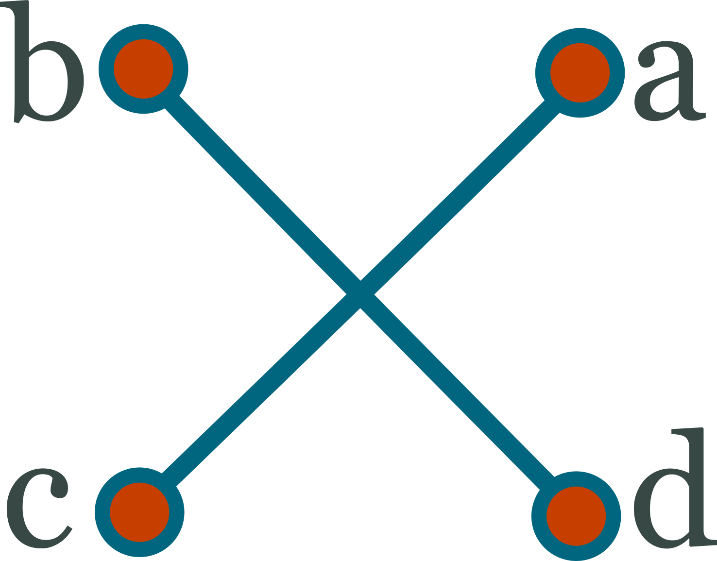
We represent each lattice with $4$ vectors, each containing is stored in its
own matrix. This means that `a[i][j]` contains the `a` vector component of the
lattice on the $i^{th}$ row and $j^{th}$ column. With this representation in
place, we perform the following to compute the next frame.
* Resolve collisions --- the collisions are performed and stored in a
temporary collision matrix.
* Propagation --- the propagation is performed and values are copied from the
temporary collision matrix into the `a`, `b`, `c`, and `d` matrices.
 \includegraphics[scale=0.1]{graphics/hpp-rep.png}
Collision
---------
Four temporary matrices are created and are called `K_a`, `K_b`, `K_c`, and
`K_d` to signify which direction they correspond to. The vector `K_a[i][j]` is
the updated based on the HPP collision rules.
One can represent the collision rules as a series of binary statements. The
best example is found in [^1] where the authors represent the collision rules
as a binary statement. Examples of the same binary statement can be found in
other papers, however (**need to record them**)
$$a = a \otimes [(a \wedge c \wedge \neg (b \vee d)) \vee (b \wedge d \wedge \neg
(a \vee c))]$$
Where the logic operator symbols are
* $\neg$ is the _not_ operator
* $\otimes$ is the _xor_ operator
* $\vee$ is the _or_ operator
* $\wedge$ is the _and_ operator
In `C`, the following code implements the above rule:
for (x = 0; x < LATTICE_WIDTH; x++) {
for (y = 0; y < LATTICE_HEIGHT; y++) {
change = (a[x][y] & c[x][y] & ~(b[x][y] | d[x][y])) |
(b[x][y] & d[x][y] & ~(a[x][y] | c[x][y]));
K_a[x][y] = a[x][y] ^ change;
K_b[x][y] = b[x][y] ^ change;
K_c[x][y] = c[x][y] ^ change;
K_d[x][y] = d[x][y] ^ change;
}
}
The boolean expression allows us to perform the computation needed without the
use of `if-else` statements. It should be also noted that we will never go
outside the bounds of the array, the same cannot be said about the propagation
step. Also note that the expression
(a1[x][y] & c1[x][y] & ~(b1[x][y] | d1[x][y])) |
(b1[x][y] & d1[x][y] & ~(a1[x][y] | c1[x][y]))
Is repeated four times in the binary representation, which is why we store it
in a separate value to reduce three computations.
Propagation
-----------
The HPP propagation step is the process of moving velocity vectors in the same
direction they are moving in after the collisions are resolved. Because of the
way we oriented our grid, we made this step unnecessarily complicated. Also
it's not clear if our representation has any advantages over a regular square
grid. Future implementation (if one is needed) would use a regular square
grid.
\includegraphics[scale=0.1]{graphics/hpp-rep.png}
Collision
---------
Four temporary matrices are created and are called `K_a`, `K_b`, `K_c`, and
`K_d` to signify which direction they correspond to. The vector `K_a[i][j]` is
the updated based on the HPP collision rules.
One can represent the collision rules as a series of binary statements. The
best example is found in [^1] where the authors represent the collision rules
as a binary statement. Examples of the same binary statement can be found in
other papers, however (**need to record them**)
$$a = a \otimes [(a \wedge c \wedge \neg (b \vee d)) \vee (b \wedge d \wedge \neg
(a \vee c))]$$
Where the logic operator symbols are
* $\neg$ is the _not_ operator
* $\otimes$ is the _xor_ operator
* $\vee$ is the _or_ operator
* $\wedge$ is the _and_ operator
In `C`, the following code implements the above rule:
for (x = 0; x < LATTICE_WIDTH; x++) {
for (y = 0; y < LATTICE_HEIGHT; y++) {
change = (a[x][y] & c[x][y] & ~(b[x][y] | d[x][y])) |
(b[x][y] & d[x][y] & ~(a[x][y] | c[x][y]));
K_a[x][y] = a[x][y] ^ change;
K_b[x][y] = b[x][y] ^ change;
K_c[x][y] = c[x][y] ^ change;
K_d[x][y] = d[x][y] ^ change;
}
}
The boolean expression allows us to perform the computation needed without the
use of `if-else` statements. It should be also noted that we will never go
outside the bounds of the array, the same cannot be said about the propagation
step. Also note that the expression
(a1[x][y] & c1[x][y] & ~(b1[x][y] | d1[x][y])) |
(b1[x][y] & d1[x][y] & ~(a1[x][y] | c1[x][y]))
Is repeated four times in the binary representation, which is why we store it
in a separate value to reduce three computations.
Propagation
-----------
The HPP propagation step is the process of moving velocity vectors in the same
direction they are moving in after the collisions are resolved. Because of the
way we oriented our grid, we made this step unnecessarily complicated. Also
it's not clear if our representation has any advantages over a regular square
grid. Future implementation (if one is needed) would use a regular square
grid.
 \includegraphics[scale=0.2]{graphics/hpp-grid.png}
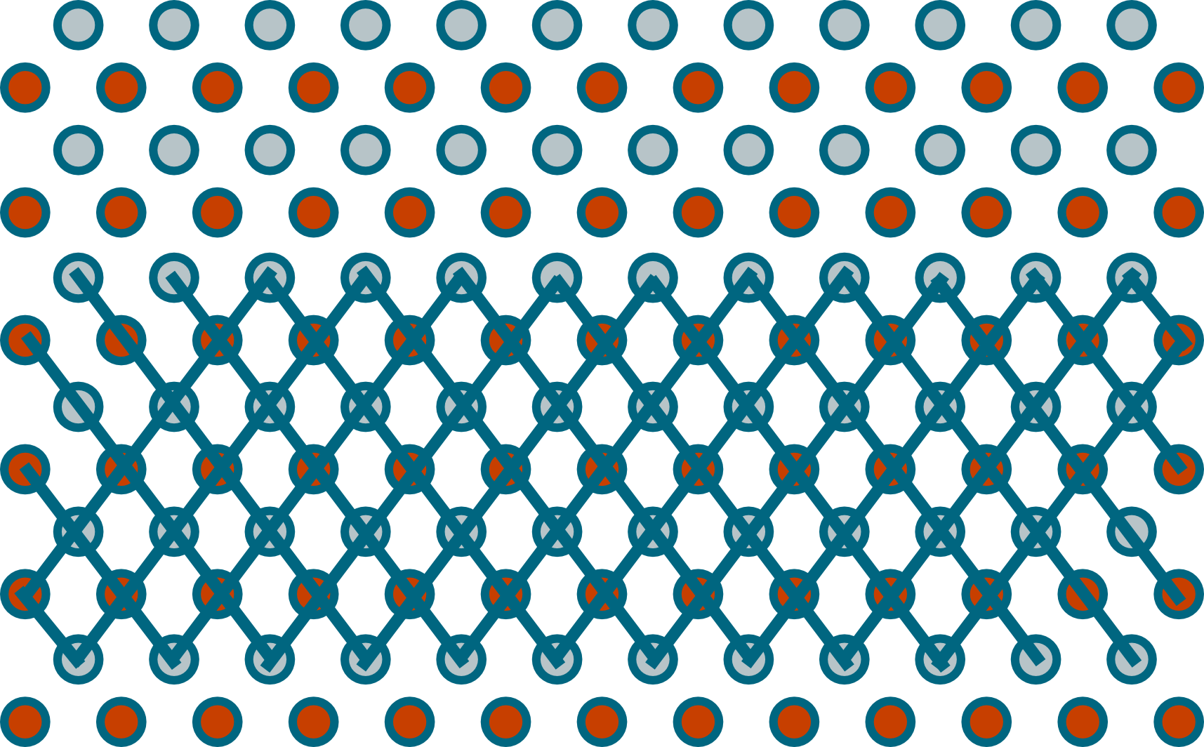
We use the following code to propagation the vectors in the lattice
a[i][j] = K_a[i-1][j-1];
b[i][j] = K_b[i-1][j+1];
c[i][j] = K_c[i+1][j+1];
d[i][j] = K_d[i+1][j-1];
it should be evident that we will run out of bounds if we run the above piece
of code over the width of the lattice array. Since we do not want to enforce
any boundary conditions at this stage of the process, we place our lattice on
a toroidal surface. This can be easily implement in `C` by noting that the
following way to access and store array elements creates the toroidal surface:
t[(i+n + LATTICE_HEIGHT) % LATTICE_HEIGHT][(j+m + LATTICE_WIDTH) % LATTICE_WIDTH]
and will also always be in the bounds of the matrix representation.
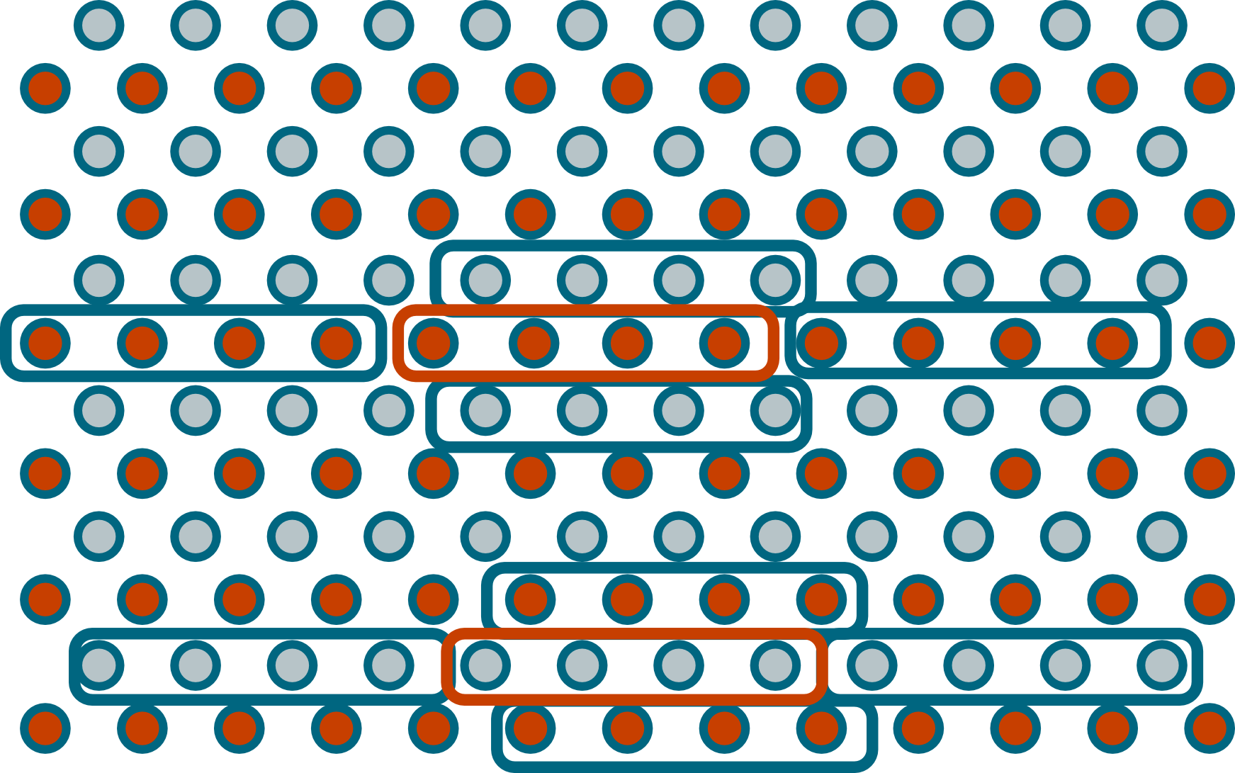
Optimizations
-------------
Since C has no differentiation between a boolean value and a short, we can
overload a short variable to contain multiple vector values. The boolean
expression does not change, but as you see from the figure below, the
propagation step has to.
\includegraphics[scale=0.2]{graphics/hpp-grid.png}
We use the following code to propagation the vectors in the lattice
a[i][j] = K_a[i-1][j-1];
b[i][j] = K_b[i-1][j+1];
c[i][j] = K_c[i+1][j+1];
d[i][j] = K_d[i+1][j-1];
it should be evident that we will run out of bounds if we run the above piece
of code over the width of the lattice array. Since we do not want to enforce
any boundary conditions at this stage of the process, we place our lattice on
a toroidal surface. This can be easily implement in `C` by noting that the
following way to access and store array elements creates the toroidal surface:
t[(i+n + LATTICE_HEIGHT) % LATTICE_HEIGHT][(j+m + LATTICE_WIDTH) % LATTICE_WIDTH]
and will also always be in the bounds of the matrix representation.
Optimizations
-------------
Since C has no differentiation between a boolean value and a short, we can
overload a short variable to contain multiple vector values. The boolean
expression does not change, but as you see from the figure below, the
propagation step has to.
 \includegraphics[scale=0.2]{graphics/propgrid.png}
The Code
--------
There are a few differences between our implementation and the one described
above:
1. The variables are called `c1`, `c2`, `c3`, and `c4` rather than `a`, `b`,
`c`, and `d`. The temporary collision arrays have also been renamed to `k1`,
`k2`, `k3`, and `k4`.
2. Our computation of blocks of vectors at a time forces us to use
checkerboard propagation.
The crux of the code for HPP is provided bellow
int x, y;
short change;
// Resolve Collisions
for (x = 0; x < LATTICE_WIDTH; x++) {
for (y = 0; y < LATTICE_HEIGHT; y++) {
change = (a1[x][y] & c1[x][y] & ~(b1[x][y] | d1[x][y])) |
(b1[x][y] & d1[x][y] & ~(a1[x][y] | c1[x][y]));
a2[x][y] = a1[x][y] ^ change;
b2[x][y] = b1[x][y] ^ change;
c2[x][y] = c1[x][y] ^ change;
d2[x][y] = d1[x][y] ^ change;
}
}
// Propagate
for (x = 1; x < LATTICE_WIDTH - 1; x++) {
for (y = 1; y < LATTICE_HEIGHT - 1; y += 2) {
a1[x][y] = (a2[x][y - 1] >> 1) + (a2[x - 1][y - 1] << LAST);
b1[x][y] = b2[x][y - 1];
c1[x][y] = c2[x][y + 1];
d1[x][y] = (d2[x][y + 1] >> 1) + (d2[x - 1][y + 1] << LAST);
a1[x][y + 1] = a2[x][y];
b1[x][y + 1] = (b2[x][y] << 1) + (b2[x + 1][y] >> LAST);
c1[x][y + 1] = (c2[x][y + 2] << 1) + (c2[x + 1][y + 2] >> LAST);
d1[x][y + 1] = d2[x - 1][y + 2];
}
}
CUDA
----
Never implemented.
FHP Model
=========
Collision
---------
Propagation
-----------
The Code
--------
Optimizations
-------------
CUDA
----
FCHC Model
==========
In the _Face Centered Hyper Cubic_ model, you have 24 vectors. 16 correspond
to the vertexes of the hyper cube while the other 8 correspond to the center
of the squares in the hyper cube.
Reduction
---------
Since you cannot store the entire table, you consider only states that have a
normalized momentum. The coordinates of the momentum $q$ are defined by
$$q_\alpha = \sum_{i = 0}^{24} S_i C_{i \alpha}$$
where $S_i$ is a boolean variable signifying the presence or absence of a
particle with velocity $C_i$. The momentum is normalized if the coordinates
satisfy
$$q_1 > q_2 > q_3 > q_4 > |q_1 - q_2 - q_3|$$
Different isometries are then applied if one of the following conditions are
satisfied in the following sequence:
* if $q_1 < 0$, then $S_1$ is applied to $q$
* if $q_2 < 0$, then $S_2$ is applied to $q$
* if $q_3 < 0$, then $S_3$ is applied to $q$
* if $q_4 < 0$, then $S_4$ is applied to $q$
* if $q_1 < q_2$, then $P_{12}$ is applied to $q$
* if $q_3 < q_4$, then $P_{34}$ is applied to $q$
* if $q_1 < q_3$, then $P_{13}$ is applied to $q$
* if $q_2 < q_4$, then $P_{24}$ is applied to $q$
* if $q_2 < q_3$, then $P_{23}$ is applied to $q$
* if $q_1 + q_4 < q_2 + q_4$, then $\Sigma_1$ is applied to $q$
* if $q_1 < q_2 + q_3 + q_4$, then $\Sigma_2$ is applied to $q$
Where
* $S_\alpha$ is the symmetry with respect to the plane $x_\alpha = 0$
* $P_{\alpha \beta}$ is the symmetry with respect to the plane
$x_\alpha = x_\beta$
* $\Sigma_1$ is the symmetry with respect to the plane
$x_1 + x_4 = x_2 + x_3$
* $\Sigma_2$ is the symmetry with respect to the plane
$x_1 = x_2 + x_3 + x_4$
[^1]: Wolf-Gladrow, Dieter. Lattice-Gas Cellular Automata and Lattice Boltzmann Models: an Introduction. Santa Clara: Springer-Verlag TELOS, 2000.
([pdf][wolf.book])
[wolf.book]: ../papers/files/Wol2000c.pdf
\includegraphics[scale=0.2]{graphics/propgrid.png}
The Code
--------
There are a few differences between our implementation and the one described
above:
1. The variables are called `c1`, `c2`, `c3`, and `c4` rather than `a`, `b`,
`c`, and `d`. The temporary collision arrays have also been renamed to `k1`,
`k2`, `k3`, and `k4`.
2. Our computation of blocks of vectors at a time forces us to use
checkerboard propagation.
The crux of the code for HPP is provided bellow
int x, y;
short change;
// Resolve Collisions
for (x = 0; x < LATTICE_WIDTH; x++) {
for (y = 0; y < LATTICE_HEIGHT; y++) {
change = (a1[x][y] & c1[x][y] & ~(b1[x][y] | d1[x][y])) |
(b1[x][y] & d1[x][y] & ~(a1[x][y] | c1[x][y]));
a2[x][y] = a1[x][y] ^ change;
b2[x][y] = b1[x][y] ^ change;
c2[x][y] = c1[x][y] ^ change;
d2[x][y] = d1[x][y] ^ change;
}
}
// Propagate
for (x = 1; x < LATTICE_WIDTH - 1; x++) {
for (y = 1; y < LATTICE_HEIGHT - 1; y += 2) {
a1[x][y] = (a2[x][y - 1] >> 1) + (a2[x - 1][y - 1] << LAST);
b1[x][y] = b2[x][y - 1];
c1[x][y] = c2[x][y + 1];
d1[x][y] = (d2[x][y + 1] >> 1) + (d2[x - 1][y + 1] << LAST);
a1[x][y + 1] = a2[x][y];
b1[x][y + 1] = (b2[x][y] << 1) + (b2[x + 1][y] >> LAST);
c1[x][y + 1] = (c2[x][y + 2] << 1) + (c2[x + 1][y + 2] >> LAST);
d1[x][y + 1] = d2[x - 1][y + 2];
}
}
CUDA
----
Never implemented.
FHP Model
=========
Collision
---------
Propagation
-----------
The Code
--------
Optimizations
-------------
CUDA
----
FCHC Model
==========
In the _Face Centered Hyper Cubic_ model, you have 24 vectors. 16 correspond
to the vertexes of the hyper cube while the other 8 correspond to the center
of the squares in the hyper cube.
Reduction
---------
Since you cannot store the entire table, you consider only states that have a
normalized momentum. The coordinates of the momentum $q$ are defined by
$$q_\alpha = \sum_{i = 0}^{24} S_i C_{i \alpha}$$
where $S_i$ is a boolean variable signifying the presence or absence of a
particle with velocity $C_i$. The momentum is normalized if the coordinates
satisfy
$$q_1 > q_2 > q_3 > q_4 > |q_1 - q_2 - q_3|$$
Different isometries are then applied if one of the following conditions are
satisfied in the following sequence:
* if $q_1 < 0$, then $S_1$ is applied to $q$
* if $q_2 < 0$, then $S_2$ is applied to $q$
* if $q_3 < 0$, then $S_3$ is applied to $q$
* if $q_4 < 0$, then $S_4$ is applied to $q$
* if $q_1 < q_2$, then $P_{12}$ is applied to $q$
* if $q_3 < q_4$, then $P_{34}$ is applied to $q$
* if $q_1 < q_3$, then $P_{13}$ is applied to $q$
* if $q_2 < q_4$, then $P_{24}$ is applied to $q$
* if $q_2 < q_3$, then $P_{23}$ is applied to $q$
* if $q_1 + q_4 < q_2 + q_4$, then $\Sigma_1$ is applied to $q$
* if $q_1 < q_2 + q_3 + q_4$, then $\Sigma_2$ is applied to $q$
Where
* $S_\alpha$ is the symmetry with respect to the plane $x_\alpha = 0$
* $P_{\alpha \beta}$ is the symmetry with respect to the plane
$x_\alpha = x_\beta$
* $\Sigma_1$ is the symmetry with respect to the plane
$x_1 + x_4 = x_2 + x_3$
* $\Sigma_2$ is the symmetry with respect to the plane
$x_1 = x_2 + x_3 + x_4$
[^1]: Wolf-Gladrow, Dieter. Lattice-Gas Cellular Automata and Lattice Boltzmann Models: an Introduction. Santa Clara: Springer-Verlag TELOS, 2000.
([pdf][wolf.book])
[wolf.book]: ../papers/files/Wol2000c.pdf